Numerical analysis using Scilab: Solving nonlinear equations

Nonlinear equations www.openeering.com page 1/25
NUMERICAL ANALYSIS USING SCILAB:
SOLVING NONLINEAR EQUATIONS
In this tutorial we provide a collection of numerical methods for solving nonlinear
equations using Scilab.
Level
This work is licensed under a Creative Commons Attribution-NonCommercial-NoDerivs 3.0 Unported License.

Step 1: The purpose of this tutorial
The purpose of this Scilab tutorial is to provide a collection of numerical
methods for finding the zeros of scalar nonlinear functions. The methods
that we present are:
 Bisection;
 Secant;
 Newton-Raphson;
 Fixed point iteration method.
These classical methods are typical topics of a numerical analysis course
at university level.
An introduction to
NUMERICAL ANALYSIS USING SCILAB
solving nonlinear equations
Step 2: Roadmap
This tutorial is composed of two main parts: the first one (Steps 3-10)
contains an introduction about the problem of solving nonlinear equations,
presents some solution strategies and introduces properties and issues of
such problems and solutions. The second part (Steps 11-23) is dedicated
to the specific methods, equipped with many Scilab examples.
Descriptions Steps
Introduction and solution strategies 3-6
Conditioning and convergence 7-10
Bisection method 11-12
Secant method 13-14
Newton method 15-18
Fixed point iteration method 19-22
Conclusions and remarks 23-25

Step 3: Introduction
Many problems that arise in different areas of engineering lead to the
solution of scalar nonlinear equations of the form
( )
i.e. to find a zero of a nonlinear function.
Nonlinear equations can have none, one, two, or an infinite number of
solutions. Some examples are presented on the right.
Note: A special class of nonlinear equations is constituted by polynomials
of the form
( ) .
(Linear chirp function ( ( )) with infinite zeros)
(Function ( ) ( ) with one zero)
The code of the examples is available in the file ex1.sce

Step 4: Solution strategies
Many solution methods exist and the correct choice depends on the type
of function . For example, different methods are used whether is a
polynomial or it is a continuous function whose derivatives are not
available.
Moreover, the problem can be stated in equivalent formulations. For
example, the original formulation ( ) can be converted into a fixed
point formulation of the form ( ) or into a minimization problem of
the form ( ).
It is important to note that even if these formulations are mathematically
equivalent (their zeros are the same ones), the numerical methods used
to approximate the solution do not have all the same behavior.
Hence, the numerical solution strategy should take into account the kind
of problem we try to solve.
Example of equivalent formulations:
Original problem:
( )
Examples of fixed point formulation:
or
( )
Example of minimization formulation:
( )

Step 5: Graphical interpretation and separation of zeros
The first step of many numerical methods for solving nonlinear equations
is to identify a starting point or an interval where to search a single zero:
this is called “separation of zeros”. If no other information is available, this
can be done by evaluating the function at several values and plotting
the results ( ).
Solving the problem ( ) is equivalent to find the solutions of the
following system
{
( )
i.e., graphically, to determine, in a Cartesian plane, the intersections of the
graph of the function ( ) with the -axis.
In the case of fixed point formulation ( ) its graphical formulation is
related to the system
{
( )
i.e. the solutions are given by the intersections of the function ( )
with the bisector .
(Separation of zeros of the original problem: )
(Fixed point equivalent formulation: ( ))
The code of the example is available in the file ex2.sce

Step 6: Example of a bracketing strategy
Bracketing is an automatic strategy for finding intervals containing a zero
of a given function . An example of bracketing is given in the following
lines of code; the idea is to identify the points in which the function
changes sign:
function xsol=fintsearch(f, xmin, xmax, neval)
// Generate x vector
x = linspace(xmin, xmax, neval)';
// Evaluate function
y = f(x);
// Check for zeros
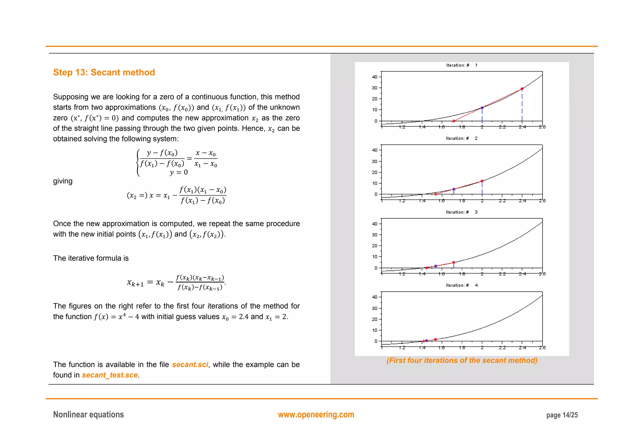
indz = find(abs(y)<=1000*%eps);
y(indz) = 0;
// Compute signs
s = sign(y);
// Find where f changes sign
inds = find(diff(s)~=0);
// Compute intervals
xsol = [x(inds),x(inds+1)];
endfunction
The code is also available in the file fintsearch.sci, while the example
can be found in fintsearch_test.sce.
(Separation of zeros for the function ( ) ( ))

Step 7: Conditioning of a zero-ﬁnding problem
The conditioning of a zero-finding problem is a measure of how it is
sensitive to perturbations of the equation.
Here we denote by a zero of the function ( ), i.e. ( ) .
From the first figure on the right we can intuitively see that if the derivative
| ( )| is “large” the problem is well-conditioned. In this case we can
clearly identify the zero of , even if there are rounding errors. Conversely,
if the derivative is “small”, the zero-finding problem is said to be ill-
conditioned and there is no clear identification of the zero. In this case, if
rounding errors are present, the zero is spread up over a “large” interval of
uncertainty.
In summary, we can state the following:
 The conditioning number of the root finding problem is | ( )|;
 The problem is ill-conditioned if | ( )| is large, i.e. | ( )| is
small.
In the graphic on the right down we can see that the zero of
( ) can not be identified because
of ill-conditioning.
(Example of well- and il- conditioned root finding problem)
(Given a very ill-conditioned problem, the unique zero cannot be
identified)

Estimating the conditioning of the problem of finding a (single) zero of a
(continuously differentiable) function ( ) means to provide an estimate of
the relative error of a perturbed solution.
Finding the zero of a function ( ), i.e. ( ) , is equivalent (for
continuously differentiable functions) to solving the inverse problem
( ).
If we consider a perturbed solution ̃, i.e. ( ̃) or, equivalently,
̃ ( ), making an error on its evaluation, we have the following
error:
̃ ( ) ( )
Using the following Taylor expansion
( ) ( ) ( ( )) ( )
and the elation obtained on the right
( ( ))
( )
the error can be written as
( ) ( ( )) ( ) ( ( ))
( )
Hence, the relative error can be stated as
| | |
( )
| | |
The code of the example on the right is available in the file ex4.sce
Original problem:
Find such that ( ) i..e. ( )
Perturbed problem:
Find ̃ such that ( ̃) i..e. ̃ ( )
Inverse function:
(Example of inverse function)
The function and its inverse are related from the relation
( ( )) ( ( ))
and the derivative of the inverse function satisfies the relation
( ( )) ( ) i.e. ( ( ))
( )
(where ( ))

Step 8: Convergence rates of iterative methods
Typically, methods for approximating nonlinear equations are based on
iterative strategies, i.e. starting from an initial guess solution , and
computing a sequence of solutions that converge to the desired
solution (where ( ) ), i.e.
We define the rate of convergence of the sequence as
| |
| |
| |
| |
for some constant and . is called the asymptotic error
constant while is the error at the iteration.
If and the convergence is called linear. We require to
ensure the convergence of the method indeed the error must be reduced
at each iteration as explained by this relation:
| | | | ( | |) | | | |
Here we compare the n+1-th step error with the initial error.
If the convergence is called superlinear.
If the convergence is called quadratic.
The following figure shows a typical convergence rate profile where we can
identify three different regions:
 an exploration region: in this region there is an exploration of the
solution space trying to find an initial guess solution (starting point)
where convergence properties are guaranteed, and, moreover, there
is no significant reduction of the error;
 a convergence region: the basin of attraction of the solution;
 a stagnation region: this last region is due to round-off errors of the
floating point system that are unavoidable.
This figure stresses the fact that the definition of the convergence rate is
valid only “in the convergence region”, hence it is a local definition.
(Typical behavior of a convergence rate profile)

Step 9: Examples of convergence rates
Let us suppose we are looking for the zero .
Linear rate:
Consider the following error model:
and
In this case we get the following errors:
zero significant figures
one significant figures
two significant figures
three significant figures
With a linear rate of convergence, the number of significant figures the
method gains is constant at each step (a multiple of the iteration number).
Quadratic rate:
Consider the following error model:
and
In this case we get the following errors:
zero significant figures
one significant figures (one
figure gained)
three significant figures (two
figures gained)
seven significant figures
(four figures gained)
With a quadratic rate of convergence, the number of significant figures the
method gains at each iteration is twice the previous iteration.
A comparison of the typical rate of convergence (when rounding errors are
present) is shown in the following figure:
(Comparison between linear, superlinear and quadratic rate of
convergence)
The number of figures gained per iteration can be summarized in the
following table:
Convergence rate Figures gained per iteration
Linear Constant
Superlinear Increasing
Quadratic Double

Step 10: Convergence criteria
When we approximate a solution with an iterative method it is necessary
to choose how to properly stop the algorithm and hence provide the
solution. As each evaluation of the function can be computationally
expensive, it is important to avoid unnecessary evaluations (for instance,
avoiding evaluations in the stagnation region).
The convergence criteria reported on the right refer to the following
problem:
 Find a solution such that ( ) starting from an initial guess
( ( )), with in .
The design criteria are based on the absolute or relative error for the
variable or for the value of the function . The difference between a
criterion based on or depends on the conditioning of the nonlinear
problem, while a choice based on the absolute or relative error depends
on the scaling of the nonlinear equations.
In our example, we consider the relative errors for f and x they are
adimensional, i.e. they allow to avoid multiplicative constants.
Example of convergence criteria:
 Absolute error between two iterates on :
| |
 Relative error between two iterates on :
| |
 Absolute residual on :
| ( )|
 Relative residual on :
| ( )| ( )
Example of implementation of a stopping criterion:
// Check for convergence
if (abs(fxnew)/fref < ftol) | (abs(dx)/xref < xtol)
// The root is found
x = xnew;
fx = fxnew;
end
The code checks the convergence both on and . If we are dealing with an
ill-conditioned problem it is likely that will not converge, so the check on
will stop the iterative method.

Step 11: Bisection method
Supposing we are looking for a zero of a continuous function, this method
starts from an interval [a,b] containing the solution and then evaluates the
function at the midpoint m=(a+b)/2. Then, according to the sign of the
function, it moves to the subinterval [a,m] or [m,b] containing the solution
and it repeats the procedure until convergence.
The main pseudo-code of the algorithm is the following:
Algorithm pseudo-code
while ((b - a) > tol) do
m = (a + b)/2
if sign(f(a)) = sign(f(m)) then
a = m
else
b = m
end
end1
The figure on the right refers to the first 4 iterations of the bisection
method applied to the function ( ) in the interval [1,2]. The
method starts from the initial interval [a,b]=[1,2] and evaluates the function
at the midpoint m=1.5. Since the sign of the function in m=1.5 is equal to
the sign of the function in b=2, the method moves to the interval
[a,m]=[1,1.5], which contains the zero. At the second step, it starts from
the interval [a,b]=[1,1.5], it evaluates the function at the midpoint m=1.25
and it moves to the interval [1.25, 1.5]. And so on.
The function is available in the file bisection.sci, while the example can
be found in bisection_test.sce. (Example of the first four iterations of the bisection method)

Step 12: Convergence of the bisection method
At each iteration of the method the searching interval is halved (and
contains the zero), i.e.
( ) ( )
Hence, the absolute error at the nth iteration is
| | | |
( )
( )
and the converge | | is guaranteed for .
Observe that at each iteration the interval is halved, i.e. ( )
( )
, but this relation does not guarantee that | | | | (i.e.
monotone convergence to ) as explained in the figure below.
However, we define the rate of the convergence for this method linear.
The figure on the right shows the relative error related to the iterations
(reported in the table below) of the method applied to the function
( ) in the interval [1,2] where the analytic solution is √ . As
expected, the method gains 1 significant figure every 3/4 iterations.
(Relative error of the bisection method)
(Iterations of the bisection method)

Step 13: Secant method
Supposing we are looking for a zero of a continuous function, this method
starts from two approximations ( , ( )) and ( ( )) of the unknown
zero ( ( ) ) and computes the new approximation as the zero
of the straight line passing through the two given points. Hence, can be
obtained solving the following system:
{
( )
( ) ( )
giving
( )
( )( )
( ) ( )
Once the new approximation is computed, we repeat the same procedure
with the new initial points ( ( )) and ( ( )).
The iterative formula is
( )( )
( ) ( )
.
The figures on the right refer to the first four iterations of the method for
the function ( ) with initial guess values and .
The function is available in the file secant.sci, while the example can be
found in secant_test.sce.
(First four iterations of the secant method)

Step 14: Convergence of the secant method
Algorithm
xkm1 = x0; fkm1 = f(x0) // Step: k-1
xk = x1; fk = f(x1) // Step: k
xkp1 = xk // Initialization
iter = 1 // Current iteration
while iter <= itermax do
iter = iter+1
xkp1 = xk-(fk*(xk-xkm1))/(fk-fkm1)
if abs(xkp1-xk)<tol break // Converg. test
xkm1 = xk; fkm1 = fk
xk = xkp1; fk = f(xkp1)
end
The algorithm iterates until convergence or until the maximum number of
iterations is reached. At each iteration only one function evaluation is
required. The “break” statement terminates the execution of the while
loop.
For the secant method it is possible to prove the following result: if the
function is continuous with continuous derivatives until order 2 near the
zero, the zero is simple (has multiplicity 1) and the initial guesses and
are picked in a neighborhood of the zero, then the method converges
and the convergence rate is equal to
√
(superlinear).
( ) in the interval [1,2], where the analytic solution is √ .
(Relative error of the secant method)
(Iterations of the secant method)

Step 15: Newton method
Supposing we are looking for a zero of a continuous function with
continuous derivatives, this method starts from an approximation of the
unknown zero and computes the new approximation as the zero of
the straight line passing through the initial point and tangent to the
function. Hence, can be obtained solving the following system:
{
( ) ( ) ( )
giving
( )
( )
( )
Once the new approximation is computed, we repeat the same procedure
with the new initial point . The iterative formula is then
( )
( )
.
The figures on the right refer to the first four iterations of the method for
the function ( ) with initial guess value .
The function is available in the file newton.sci, while all the examples
related to this method can be found in newton_test.sce.
(First four iterations of the Newton method)

Step 16: Convergence of the Newton method
Algorithm
xk = x0;
iter = 1 // Current iteration
while iter <= itermax do
iter = iter+1
xkp1 = xk-f(xk)/f’(xk)
if abs(xkp1-xk)<tol break // Converg. test
xk = xkp1;
end1
The algorithm iterates until convergence or the maximum number of
iterations is reached. At each iterations a function evaluation with its
derivative is required. The “break” statement terminates the execution of
the while loop.
For the newton method it is possible to prove the following results: if the
function f is continuous with continuous derivatives until order 2 near the
zero, the zero is simple (has multiplicity 1) and the initial guess is
picked in a neighborhood of the zero, then the method converges and the
convergence rate is equal to (quadratic).
( ) in the interval [1,2], where the analytic solution is √ . As
expected, the number significant figures doubles at each iteration.
(Relative error of the Newton method)
(Iterations of the Newton method)

Step 17: Newton method (loss of quadratic convergence)
A zero is said to be multiple with multiplicity if
( ) ( ) ( ) and ( ) .
In the Newton method, if the zero is multiple, the convergence rate
decreases from quadratic to linear. As an example, consider the function
( ) with zero . Then the Newton method can be stated as
giving the error
which is clearly linear.
On the right we report an example of loss of quadratic convergence
applied to the function
( ) ( )
which has a zero of multiplicity 2 in .
The relative error shows a linear behavior, indeed the method gains a
constant number of significant figures every 3 or 4 iterations.
(Function with a zero of multiplicity 2)
(Loss of quadratic convergence)

Step 18: Newton method (Global convergence)
If the function of which we are looking for the zeros and its derivatives until
order 2 are continuous, it is possible to ensure the global convergence of
the Newton method by choosing a proper initial guess point.
As reported in the table on the right, under the above mentioned
hypothesis it is possible to identify a neighborhood of the zero such
that, for each initial guess in , the sequence is monotonically
decreasing (or increasing) to the zero.
For instance, if the function is convex and increasing (second row and
second column case in the table), the Newton method with an initial guess
picked on the right of the zero converges monotonically decreasing to the
unknown zero.
The Newton method with the above choosing criterion also ensures that
all are well defined, i.e. the method does not generate any point in
which the function is not defined (an example in which the monotonicity of
the convergence is important is the logarithm function, which is not
defined for negative values).
Function
properties
( )
(decrease)
( )
(increase)
( )
(concave)
(Right domain) (Left domain)
( )
(convex)
(Left domain) (Right domain)
(How to choose the initial guess for global convergence)

Step 19: Fixed point iteration method
The fixed point iteration method transforms the original problem ( )
into the problem ( ) and solves it using an iterative scheme of the
form:
( ).
If the iterative scheme converges to the value , i.e. ( ), then is
also a zero of ( ), since ( ) ( ) .
Solving the equation ( ) is equivalent to solve the following system
{
( )
On the right we reported some graphical examples of iterations applied to
6 different functions . The three examples on the left show cases in
which the method converges to the unknown zero, while among the
examples on the right there is no convergence of the method, even if the
functions seem to be quite similar to the ones on the left.
Note: The Newton method is a particular case of fixed point iteration
method where ( )
( )
( )
.
(Graphical examples of iterations applied to 6 different functions )

Step 20: Fixed point iteration method - example #1
The example on the right refers to the function ( ) , where the
considered fixed point iteration is
( )
Here the relative error shows a linear behavior of the method, while on the
right we can see the first four iterations of the method.
(Relative error and iterations of the fixed point iteration method)
The function is available in the file fixedpoint.sci, while the example can
be found in fixedpoint_test.sce.
(First four iterations of the fixed-point iteration method))

Step 21: Convergence of the fixed point iteration method
It is possible to prove that the sequence converges to if
| ( )| (i.e. it is a contraction) in the interval containing the
initial guess and for all (i.e. ( ) ). Moreover, in this case, it is
possible to prove that the solution is the unique solution in the interval
of the equation ( ) . While, if | ( )| in the whole interval , the
sequence does not converge to the solution (even if we start very close to
the zero ).
The convergence rate of the fixed point iteration method is:
 If ( ) , the method has a linear convergence rate;
 If ( ) and ( ) , the method has a quadratic
convergence rate;
Example: The fixed point iteration method applied to the Newton method
with fixed point function
( )
( )
( )
with ( ) and ( ) shows a quadratic rate of convergence,
indeed we have ( ) and ( ) ( ( )
( ) ( ) ( ) ( )
( ( ))
).
Proof of convergence (idea)
Using the Taylor formula we have
( ) ( ) ( ) ( ) ( )
( ) ( ) ( ) ( ) ( )
( ) ( ) ( ) ( ) ( )
where are unknown values in the intervals ( ). If the derivatives are
bounded by the relation
| ( )|
the error can be written as
| | ( ) | |
i.e.
| | | |
where is the initial error.
Proof of convergence rate (idea)
Assuming ( ) and using the Taylor formula we have
( ) ( )
( ) ( ) ( )
( )
( )
( )
( )
where ( ) and ( ).
If ( ) we have a linear rate of convergence of the sequence, i.e.
| |
| |
( ).
If ( ) and ( ) we have a quadratic rate of convergence of the
sequence, i.e.
| |
| |
( ).

Step 22: Fixed point iteration method - example #2
This example refers to the zero of the function
( )
which is .
Starting from this function it is possible to write different kinds of fixed
point iterations:
1. with ( ) : This function shows a linear
behavior of convergence (blue line), indeed the derivative
( ) ;
2. ( ) with ( ) ( ) : This function does not
converge (red line), indeed the derivative ( ) ;
3. with ( ) : This function shows a quadratic
rate of convergence (purple line), indeed the derivative ( ) .
The initial guess is equal to .
Also this second example can be found in the file fixedpoint_test.sce.
(Original function)
(Relative error for different fixed point iterations)

Step 23: Comparison of the methods – an example
This example refers to the zero of the function
( ) ( )
which is .
In the figure on the right we can see a typical result on relative errors, in
step with the rates of convergence discussed earlier for the different
methods.
At a first glance, one might think that the Newton method should be
always chosen, since its convergence is the best one, but it has to be
considered that this method needs the computation of the derivative,
which could require the evaluation of the original function, which can be
numerically very expensive.
The source code of this example can be found in the file main_fcn.sce.
(Nonlinear test function)
(Relative error of the 4 methods)

Step 24: Concluding remarks and References
In this tutorial we have collected a series of numerical examples written in
Scilab to tackle the problem of finding the zeros of scalar nonlinear
equations with the main methods on which are based the state-of-the-art
algorithms.
On the right-hand column you may find a list of references for further
studies.
1. Scilab Web Page: www.scilab.org.
2. Openeering: www.openeering.com.
3. K. Atkinson, An Introduction to Numerical Analysis, John Wiley, New
York, 1989.
Step 25: Software content
To report a bug or suggest some improvement please contact the
Openeering team at the web site www.openeering.com.
Thank you for your attention,
Anna Bassi and Manolo Venturin
--------------
Main directory
--------------
ex1.sce : Examples of zero-finding problems
ex2.sce : Examples of separation and fixed point
ex3.sce : Example on conditioning
ex4.sce : Example of inverse function
ex5.sce : Examples of convergence rates
fintsearch.sci : Search intervals
fintsearch_test.sce: Test for search intervals
bisection.sci : Bisection method
bisection_test.sce : Test for the bisection method
secant.sci : Secant method
secant_test.sce : Test for the secant method
newton.sci : Newton-Raphson method
newton_test.sce : Test for the Newton-Raphson method
fixedpoint.sci : Fixed point iteration method
fixedpoint_test.sce: Tests for the fixed point iteration method
main_fcn.sce : Comparison of methods
license.txt : License file

Numerical analysis using Scilab: Solving nonlinear equations

More Related Content

What's hot

Viewers also liked

Similar to Numerical analysis using Scilab: Solving nonlinear equations

More from Scilab

Recently uploaded

Numerical analysis using Scilab: Solving nonlinear equations