1. The document provides information about a numerical methods course for physics majors at Vivekananda College in Tiruvedakam West, including the reference textbook and details about Unit V on numerical solutions of ordinary differential equations.
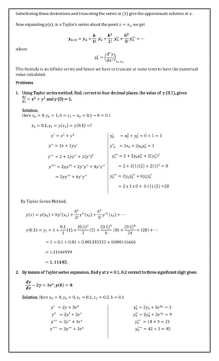
2. It introduces the concept of using Taylor series approximations to find numerical solutions to differential equations, providing the general Taylor series expansion formula and explaining how to derive the terms needed to solve specific differential equations.
3. It gives examples of using the Taylor series method to solve sample ordinary differential equations, finding approximate values of y at increasing values of x to several decimal places.
![VIVEKANANDA COLLEGE, TIRUVEDAKAM WEST
(Residential & Autonomous – A Gurukula Institute of Life-Training)
(Affiliated to Madurai Kamaraj University)
PART III: PHYSICS MAJOR – FOURTH SEMESTER-CORE SUBJECT PAPER-II
NUMERICAL METHODS – 06CT42
(For those who joined in June 2018 and after)
Reference Text Book: Numerical Methods – P.Kandasamy, K.Thilagavathy & K.Gunavathi,
S.Chand & Company Ltd., New Delhi, 2014.
UNIT – V NUMERICAL SOLUTION OF ORDINARY DIFFERENTIAL EQUATIONS
Introduction:
In solving a differential equation for approximate solution. We find numerical values of
𝑦1, 𝑦2, 𝑦3 …. corresponding to given numerical values of independent variable values 𝑥1, 𝑥2, 𝑥3 … so
that the orderd pairs (𝑥𝑖, 𝑦𝑖), (𝑥2, 𝑦2) … … satisfy a particular solution, though approximately. A
solution of this type is called a point wise solution. Suppose we require to sole
𝑑𝑦
𝑑𝑥
= 𝑓(𝑥, 𝑦) with the
initial condition 𝑦(𝑥0) = 𝑦0. By numerical solution of the differential equation, let 𝑦(𝑥0) =
𝑦0, 𝑦(𝑥1), 𝑦(𝑥2), … be the solution of y at 𝑥 = 𝑥0, 𝑥1, 𝑥2, … Let 𝑦 = 𝑦(𝑥)be the exact solution.
Truncation errors are the errors that result from using an approximation in place of an exact
mathematical procedure. at 𝑥 = 𝑥𝑖
Power Series approximations
Let us suppose that we require to find the solution of
𝑦′
=
𝑑𝑦
𝑑𝑥
= 𝑓(𝑥, 𝑦)
subject to the initial condition 𝑦(𝑥0) = 𝑦0
By Taylor series, we have
𝑦(𝑥) = 𝑦(𝑥0) +
𝑥 − 𝑥0
1!
𝑦′(𝑥0) +
(𝑥 − 𝑥0)2
2!
𝑦′′(𝑥0) + ⋯
If 𝑥 = 𝑥0 = 0 (origin) we get the Maclaurin series expansion,
𝑦(𝑥) = 𝑦(0) +
𝑥
1!
𝑦′(0) +
𝑥2
2!
𝑦′′(0) + ⋯
Solution by Taylor series (Type 1)
If 𝑦′
= 𝑓(𝑡, 𝑦)𝑥0 ≤ 𝑥 ≤ 𝑏 𝑤𝑖𝑡ℎ 𝑦(𝑡0) = 𝑦0 gives the solution 𝑦0 at initial point 𝑥 = 𝑥0 for given step
size ℎ, the solution at 𝑥 = 𝑥0 + ℎ 𝑜𝑟 ℎ = 𝑥1 − 𝑥0 can be computed from Taylor series as
𝑦(𝑥) = 𝑦(𝑥0 + ℎ) = 𝑦(𝑥0) + ℎ𝑦′(𝑥0) +
ℎ2
2!
𝑦′′(𝑥0) +
ℎ3
3!
𝑦′′′(𝑥0) + ⋯ … (1)
from the differential equation, if is observed that 𝑦′(𝑥0) = 𝑓(𝑥0, 𝑦0)
Repeated differentiation gives 𝑦′′(𝑥0), 𝑦′′′(𝑥0) …as
𝑦′′(𝑥0) = [
𝛿𝑓
𝛿𝑡
+
𝛿𝑓
𝛿𝑦
𝑦′
]
𝑥=𝑥0
𝑦′′′(𝑥0) = [
𝛿2
𝑓
𝑑𝑡2
+
2𝛿2
𝑓
𝛿𝑡𝛿𝑦
𝑦′
+ (
𝛿𝑓
𝛿𝑦
𝑦′
)
2
]
𝑥=𝑥0
and so on](https://image.slidesharecdn.com/unit-vnumericalsolutionofordinarydifferentialequations-200504172216/85/Study-Material-Numerical-Solution-of-Odinary-Differential-Equations-1-320.jpg)
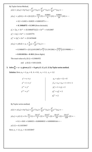
![VIVEKANANDA COLLEGE, TIRUVEDAKAM WEST
(Residential & Autonomous – A Gurukula Institute of Life-Training)
(Affiliated to Madurai Kamaraj University)
PART III: PHYSICS MAJOR – FOURTH SEMESTER-CORE SUBJECT PAPER-II
NUMERICAL METHODS – 06CT42
(For those who joined in June 2018 and after)
Reference Text Book: Numerical Methods – P.Kandasamy, K.Thilagavathy & K.Gunavathi,
S.Chand & Company Ltd., New Delhi, 2014.
UNIT – V NUMERICAL SOLUTION OF ORDINARY DIFFERENTIAL EQUATIONS
Introduction:
In solving a differential equation for approximate solution. We find numerical values of
𝑦1, 𝑦2, 𝑦3 …. corresponding to given numerical values of independent variable values 𝑥1, 𝑥2, 𝑥3 … so
that the orderd pairs (𝑥𝑖, 𝑦𝑖), (𝑥2, 𝑦2) … … satisfy a particular solution, though approximately. A
solution of this type is called a point wise solution. Suppose we require to sole
𝑑𝑦
𝑑𝑥
= 𝑓(𝑥, 𝑦) with the
initial condition 𝑦(𝑥0) = 𝑦0. By numerical solution of the differential equation, let 𝑦(𝑥0) =
𝑦0, 𝑦(𝑥1), 𝑦(𝑥2), … be the solution of y at 𝑥 = 𝑥0, 𝑥1, 𝑥2, … Let 𝑦 = 𝑦(𝑥)be the exact solution.
Truncation errors are the errors that result from using an approximation in place of an exact
mathematical procedure. at 𝑥 = 𝑥𝑖
Power Series approximations
Let us suppose that we require to find the solution of
𝑦′
=
𝑑𝑦
𝑑𝑥
= 𝑓(𝑥, 𝑦)
subject to the initial condition 𝑦(𝑥0) = 𝑦0
By Taylor series, we have
𝑦(𝑥) = 𝑦(𝑥0) +
𝑥 − 𝑥0
1!
𝑦′(𝑥0) +
(𝑥 − 𝑥0)2
2!
𝑦′′(𝑥0) + ⋯
If 𝑥 = 𝑥0 = 0 (origin) we get the Maclaurin series expansion,
𝑦(𝑥) = 𝑦(0) +
𝑥
1!
𝑦′(0) +
𝑥2
2!
𝑦′′(0) + ⋯
Solution by Taylor series (Type 1)
If 𝑦′
= 𝑓(𝑡, 𝑦)𝑥0 ≤ 𝑥 ≤ 𝑏 𝑤𝑖𝑡ℎ 𝑦(𝑡0) = 𝑦0 gives the solution 𝑦0 at initial point 𝑥 = 𝑥0 for given step
size ℎ, the solution at 𝑥 = 𝑥0 + ℎ 𝑜𝑟 ℎ = 𝑥1 − 𝑥0 can be computed from Taylor series as
𝑦(𝑥) = 𝑦(𝑥0 + ℎ) = 𝑦(𝑥0) + ℎ𝑦′(𝑥0) +
ℎ2
2!
𝑦′′(𝑥0) +
ℎ3
3!
𝑦′′′(𝑥0) + ⋯ … (1)
from the differential equation, if is observed that 𝑦′(𝑥0) = 𝑓(𝑥0, 𝑦0)
Repeated differentiation gives 𝑦′′(𝑥0), 𝑦′′′(𝑥0) …as
𝑦′′(𝑥0) = [
𝛿𝑓
𝛿𝑡
+
𝛿𝑓
𝛿𝑦
𝑦′
]
𝑥=𝑥0
𝑦′′′(𝑥0) = [
𝛿2
𝑓
𝑑𝑡2
+
2𝛿2
𝑓
𝛿𝑡𝛿𝑦
𝑦′
+ (
𝛿𝑓
𝛿𝑦
𝑦′
)
2
]
𝑥=𝑥0
and so on](https://image.slidesharecdn.com/unit-vnumericalsolutionofordinarydifferentialequations-200504172216/75/Study-Material-Numerical-Solution-of-Odinary-Differential-Equations-1-2048.jpg)
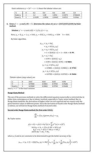
![Now, take 𝑥2 = 1.2, ℎ = 0.1
By Taylor series
𝑦(𝑥2) = 𝑦(𝑥1) + ℎ𝑦′(𝑥1) +
ℎ2
2!
𝑦′′(𝑥1) +
ℎ3
3!
𝑦′′′(𝑥1) +
ℎ4
4!
𝑦′′′′(𝑥1) + ⋯
𝑦(𝑥2) = 𝑦(1.2)
= 0.11033847 +
0.1
1
(1.21033847) +
(0.1)2
2
(2.21033847) +
(0.1)3
6
(2.21033847)
+
(0.1)4
24
(2.21033847) + ⋯
= 0.11033847 + 0.121033847 + 2.21033847(0.005 + 0.0016666 + ⋯ )
= 𝟎. 𝟐𝟒𝟐𝟖𝟎𝟏𝟔𝟎.
4. Using Taylor method, compute y(0.2) and y(0.4) correct to 4 decimal places given
𝑑𝑦
𝑑𝑥
= 1 − 2𝑥𝑦
and y(0)=0.
Solution. Here 𝑥0 = 0, 𝑦0 = 0, 𝑥1 = 0.2, 𝑥2 = 0.4, ℎ = 0.2
𝑦′
= 1 − 2𝑥𝑦
𝑦′′
= −2(𝑥𝑦′
+ 𝑦)
𝑦′′
′ = −2(𝑥𝑦′′
+ 2𝑦′)
𝑦′′′′
= −2(𝑥𝑦′′′
+ 3𝑦′′)
𝑦′′′′′
= −2(2𝑥𝑦′′′′
+ 4𝑦′′′
)
𝑦0
′
= 1 − 2𝑥0 𝑦0 = 1
𝑦0
′′
= 0
𝑦0
′′′
= −4
𝑦0
′′′′
= 0
𝑦0
′′′′′
= 32
By Taylor series.
𝑦(𝑥) = 𝑦(𝑥0) + ℎ𝑦′(𝑥0) +
ℎ2
2!
𝑦′′(𝑥0) +
ℎ3
3!
𝑦′′′(𝑥0) +
ℎ4
4!
𝑦′′′′(𝑥0) + ⋯
𝑦(𝑥1) = 𝑦(0.2) = 0 +
0.2
1
(1) +
(0.2)2
2
(0) +
(0.2)3
6
(−4) +
(0.2)4
24
(0) +
(0.2)5
120
(32) + ⋯
= 0.2 − 0.00533333 + 0.000085333
= 𝟎. 𝟏𝟗𝟒𝟕𝟓𝟐𝟎𝟎𝟑
Here, 𝑥1 = 0.2 𝑦1 = 0.194752003, ℎ = 0.2
𝑦′1 = 𝑥1 + 𝑦1
𝑦1
′′
= 1 + 𝑦1
;
𝑦1
′′′
= 𝑦1
′′
𝑦1
′′′′
= 𝑦1′′′
𝑦1
′
= 𝑥1 + 𝑦1 = 1.1 + 0.11033847 = 1.21033847
𝑦1
′′
= 1 + 1.21033847 = 2.21033847
𝑦1
′′′
= 𝑦1
′′
= 𝑦1
′′′′
= 𝑦1
′′′′′
= ⋯ = 2.21033847
𝑦1
′
= 1 − 2𝑥1 𝑦1
𝑦1
′′
= −2(𝑥1 𝑦1
′
+ 𝑦1)
𝑦1
′′′
= −2(𝑥1 𝑦1
′′
+ 2𝑦1
′)
𝑦1
′′′′
= −2(𝑥1 𝑦1
′′′
+ 3𝑦1
′′)
𝑦1
′′′′′
= −2(2𝑥1 𝑦1
′′′
+ 4𝑦1
′′′
)
𝑦1
′
= 1 − 2(0.2)(0.194752003) = 0.9220992
𝑦1
′′
= −2[(0.2)(0.9220992) + 0.194752003]
= −0.758343686
𝑦1
′′′
= −2[(0.2)(−0.758343686)
+ 2(0.9220992)]
= −3.38505933
𝑦1
′′′′
= −2[(0.2)(-3.38505933)+3(-
0.75834686)]
= 5.90408585](https://image.slidesharecdn.com/unit-vnumericalsolutionofordinarydifferentialequations-200504172216/85/Study-Material-Numerical-Solution-of-Odinary-Differential-Equations-4-320.jpg)
![Here, 𝑥2 = 0.4 ℎ = 0.2
By Taylor Series
𝑦(𝑥2) = 𝑦(𝑥1) + ℎ𝑦′(𝑥1) +
ℎ2
2!
𝑦′′(𝑥1) +
ℎ3
3!
𝑦′′′(𝑥1) +
ℎ4
4!
𝑦′′′′(𝑥1) + ⋯
𝑦(𝑥2) = 𝑦(0.4)
= 0.194752003 +
0.2
1
(0.9220992) +
(0.2)2
2
(−0.758343686) +
(0.2)3
6
(−3.38505933)
+
(0.2)4
24
(5.90403585)
= 0.194752003 + 0.18441984 − 0.0151668737 − 0.00451341243 + 0.00039360239
= 0.35988515
Euler’s Method
In solving a first order differential equation by numerical methods, we come across two types of
solutions:
• A series solution of y in terms of x, which will yield the value of y at a particular value of x
by direct substitution in the series solution.
• Values of y at specified values of x.
Let us take the point 𝑥 = 𝑥0, 𝑥1, 𝑥2, … 𝑤ℎ𝑒𝑟𝑒 𝑥1 − 𝑥𝑖−1 = ℎ 𝑖. 𝑒. , 𝑥𝑖 = 𝑥0 + 𝑖ℎ, 𝑖 = 0,1,2, ….
The equation of tangent at (𝑥0, 𝑦0) to curve is
𝑦 − 𝑦0 = 𝑦(𝑥0,𝑦0)
′
(𝑥 − 𝑥0)
= 𝑓(𝑥0, 𝑦0). (𝑥 − 𝑥0)
𝑦 = 𝑦0 + 𝑓(𝑥0, 𝑦0). (𝑥 − 𝑥0)
∴ 𝑦1 = 𝑦0 + ℎ𝑦0
′
𝑤ℎ𝑒𝑟𝑒 ℎ = 𝑥1 − 𝑥0.
Thus
𝒚 𝒏+𝟏 = 𝒚 𝒏 + 𝒉𝒇(𝒙 𝒏, 𝒚 𝒏); 𝒏 = 𝟎, 𝟏, 𝟐, …
This formula is called Euler’s algorithm
5. Using Euler’s method, solve numerically the equation, 𝒚′
= 𝒙 + 𝒚, 𝒚(𝟎) = 𝟏, 𝒇𝒐𝒓 𝒙 =
𝟎. 𝟎 (𝟎. 𝟐)(𝟏. 𝟎) Check your answer with the exact solution.
Solution. Here, h=0.2, 𝑓(𝑥, 𝑦) = 𝑥 + 𝑦, 𝑥0 = 0, 𝑦0 = 1 𝑥1 = 0.2, 𝑥2 = 0.4, 𝑥3 = 0.6, 𝑥4 =
0.8, 𝑥5 = 1.0
By Euler algorithm
𝑦1 = 𝑦0 + ℎ𝑓(𝑥0, 𝑦0)
𝑦1 = 𝑦0 + ℎ[𝑥0 + 𝑦0]
= 1 + (0.2)(0 + 1) = 𝟏. 𝟐
𝑦2 = 𝑦1 + ℎ[𝑥1 + 𝑦1]
= 1.2 + (0.2)(0.2 + 1.2) = 𝟏. 𝟒𝟖
𝑦3 = 𝑦2 + ℎ[𝑥2 + 𝑦2]
= 1.48 + (0.2)(0.4 + 1.48) = 𝟏. 𝟖𝟓𝟔
𝑦4 = 1.856 + (0.2)(0.6 + 1.856) = 𝟐. 𝟑𝟒𝟕𝟐
𝑦5 = 2.3472 + (0.2)(0.8 + 2.3472) = 𝟐. 𝟗𝟒𝟔𝟔𝟒](https://image.slidesharecdn.com/unit-vnumericalsolutionofordinarydifferentialequations-200504172216/85/Study-Material-Numerical-Solution-of-Odinary-Differential-Equations-5-320.jpg)
![From this general second order Runge-Kutta formula, setting 𝑎 = 0, 𝑏 = 1, 𝑚 =
1
2
, we get the
second order Runge-Kutta algorithm as
𝑘1 = ℎ𝑓(𝑥, 𝑦)
𝑘2 = ℎ𝑓 (𝑥 +
1
2
ℎ, 𝑦 +
1
2
𝑘1)
and ∆𝑦 = 𝐾2 where ℎ = ∆𝑥.
Since the derivation of third and fourth order Runge-Kutta algorithms are tedious, we state them
below for use.
The third order Runge-Kutta method algorithm is given below:
The fourth order Runge-Kutta method algorithm is mostly used in problem unless other
mentioned. It is
7. Using Runge-Kutta method of fourth order, solve
𝒅𝒚
𝒅𝒙
=
𝒚 𝟐−𝒙 𝟐
𝒚 𝟐+𝒙 𝟐
given
y(0)=1 at x=0.2,0.4.
Solution. 𝑦′
= 𝑓(𝑥, 𝑦) =
𝑦2−𝑥2
𝑦2+𝑥2
Here 𝑥0 = 0, ℎ = 0.2, 𝑥1 = 0.2, 𝑥2 = 0.4, 𝑦0 = 1
𝑓(𝑥0, 𝑦0) = 𝑓(0,1) =
1 − 0
1 + 0
= 1
𝑘1 = ℎ𝑓(𝑥0, 𝑦0) = (0.2)(1) = 0.2
𝑘2 = ℎ𝑓 (𝑥0 +
1
2
ℎ, 𝑦0 +
1
2
𝑘1) = (0.2)𝑓(0.1,1.1)
= (0.2) [
(1.1)2
− (0.1)2
(1.1)2 + (0.1)2
] = (0.2) [
1.21 − 0.01
1.21 + 0.01
]
= 0.1967213
𝑘3 = ℎ𝑓 (𝑥0 +
1
2
ℎ, 𝑦0 +
1
2
𝑘2)
= (0.2)𝑓 (0.1, 1 +
1
2
(0.1967213))
= (0.2)𝑓(0.1,1.0983606)
= (0.2) [
(1.0983606)2
− (0.01)
(1.0983606)2 + (0.01)
] = 0.1967
Second order R.K. algorithm
𝑘1 = ℎ𝑓(𝑥, 𝑦)
𝑘2 = ℎ𝑓 (𝑥 +
1
2
ℎ, 𝑦 +
1
2
𝑘1)
𝑘3 = ℎ𝑓(𝑥 + ℎ, 𝑦 + 2𝑘2 − 𝑘1)
and ∆𝑦 =
1
6
(𝑘1 + 4𝑘2 + 𝑘3)
Third order
R.K. algorithm
𝑘1 = ℎ𝑓(𝑥, 𝑦)
𝑘2 = ℎ𝑓 (𝑥 +
1
2
ℎ, 𝑦 +
1
2
𝑘1)
𝑘3 = ℎ𝑓(𝑥 + ℎ, 𝑦 + 2𝑘2 − 𝑘1)
𝑘4 = ℎ𝑓(𝑥 + ℎ, 𝑦 + 𝑘3)
and ∆𝑦 =
1
6
(𝑘1 + 4𝑘2 + 2𝑘3) + 𝑘4)
𝑦(𝑥 + ℎ) = 𝑦(𝑥) + ∆𝑦
Fourth order
R.K. algorithm](https://image.slidesharecdn.com/unit-vnumericalsolutionofordinarydifferentialequations-200504172216/85/Study-Material-Numerical-Solution-of-Odinary-Differential-Equations-7-320.jpg)
![𝑘4 = ℎ𝑓(𝑥0 + ℎ, 𝑦0 + 𝑘3)
= (0.2)𝑓(0.2,1.1967)
= (0.2) [
(1.1967)2
− (0.2)2
(1.1967)2 + (0.2)2
] = 0.1891
∴ ∆𝑦 =
1
6
[𝑘1 + 2𝑘2 + 𝑘4]
=
1
6
[0.2 + 2(0.19672) + 2(1.1967) + 0.1891]
= 0.19598
𝒚(𝟎. 𝟐) = 𝒚 𝟏 = 𝒚 𝟎 + ∆𝒚 = 𝟏. 𝟏𝟗𝟓𝟗𝟖
Again to find y(0.4) start form (𝑥1, 𝑦1) = (0.2, 1.19598)
Now,
∴ 𝑘1 = ℎ𝑓(𝑥1, 𝑦1) = (0.2) [
(1.19598)2
− (0.2)2
(1.19598)2 + (0.2)2
] = 0.1891
𝑘2 = ℎ𝑓 (𝑥1 +
1
2
ℎ, 𝑦1 +
1
2
𝑘1) = (0.2)𝑓(0.3,1.29055)
= (0.2) [
(1.29055)2
− (0.3)2
(1.29055)2 + (0.3)2
] = 0.17949
𝑘3 = (0.2)𝑓(0.3,1.28572) = 0.1793
𝑘4 = (0.2)𝑓(0.4, 𝑦1 + 𝑘3) = (0.2)𝑓(0.4,1.37528)
= 0.1687
∆𝑦 =
1
6
(𝑘1 + 2𝑘2 + 2𝑘3 + 𝑘4)
=
1
6
[0.1891 + 2(0.1795) + 2(0.1793) + 0.1687] = 0.1792
∴ 𝒚 𝟐 = 𝒚(𝟎. 𝟒) = 𝒚 𝟏 + ∆𝒚 = 𝟏. 𝟑𝟕𝟓𝟏.
8. Compute y(0.3) given
𝒅𝒚
𝒅𝒙
+ 𝒚 + 𝒙𝒚 𝟐
= 𝟎, y (0) =1 by taking h=0.1 using R.K method of fourth
order (correct to 4 decimals)
Solution. 𝑦′
= −(𝑥𝑦2
+ 𝑦) = 𝑓(𝑥, 𝑦); 𝑥0 = 0, 𝑦0 = 1, ℎ = 0.1, 𝑥1 = 0.1, 𝑥2 = 0.2, 𝑥3 = 0.3,
𝑦3 =?
𝑘1 = ℎ𝑓(𝑥0, 𝑦0) = (0.1)[−(𝑥0 𝑦0
2
+ 𝑦0)] = −0.1
𝑘2 = ℎ𝑓 (𝑥0 +
1
2
ℎ, 𝑦0 +
1
2
𝑘1) = (0.1)𝑓(0.05,0.95)
= −0.1[(0.05)(0.95)2
+ 0.95]
= −0.0995
𝑘3 = ℎ𝑓 (𝑥0 +
1
2
ℎ, 𝑦0 +
1
2
𝑘2)
= (0.1)𝑓(0.05,0.95025)
= (0.1)[−(0.05 𝑥 0.95025 + 1)(0.95025)]
= −0.09953987 ≈ −0.0995.](https://image.slidesharecdn.com/unit-vnumericalsolutionofordinarydifferentialequations-200504172216/85/Study-Material-Numerical-Solution-of-Odinary-Differential-Equations-8-320.jpg)
![𝑘4 = ℎ𝑓(𝑥0 + ℎ, 𝑦0 + 𝑘3)
= (0.1)𝑓(0.1,0.9005) = −0.0982.
𝑦1 = 𝑦(0.1) = 1 +
1
6
[−0.1 + 2(−0.0995) + 2(−0.0995) − 0.0982]
𝑦(0.1) = 𝟎. 𝟗𝟎𝟎𝟔.
Again taking (𝑥1, 𝑦1)in place of 𝑥0, 𝑦0) repeat the process
𝑘1 = ℎ𝑓(𝑥1, 𝑦1) = (0.1)𝑓(0.1,0.9006) = −0.0982
𝑘2 = ℎ𝑓 (𝑥1 +
1
2
ℎ, 𝑦1 +
1
2
𝑘1) = (0.1)𝑓(0.15,0.8515) = −0.0960
𝑘3 = ℎ𝑓 (𝑥1 +
ℎ
2
, 𝑦1 +
1
2
𝑘2) = (0.1)𝑓(0.15, 0.8526) = −0.0962
𝑘4 = ℎ𝑓(𝑥1 + ℎ, , 𝑦1 + 𝑘3) = (0.1)𝑓(0.2,0.8044) = −0.0934
𝑦2 = 𝑦1 +
1
6
(𝑘1 + 2𝑘2 + 2𝑘3 + 𝑘4)
𝑦2 = 𝑦(0.2) = 0.9006 +
1
6
[−0.0982 + 2(−0.0960) + 2(−0.0962) + (−0.0934)]
𝑦(0.2) = 𝟎. 𝟖𝟎𝟒𝟔
Again, starting form (𝑥2, 𝑦2) in place of (𝑥0, 𝑦0)
𝑘1 = −0.0934, 𝑘2 = −0.0902, 𝑘3 = −0.0904, 𝑘4 = −0.0867
∴ 𝑦3 = 𝑦(0.3) = 𝑦2 +
1
6
∆𝑦 = 𝑦2 +
1
6
(𝑘1 + 2𝑘2 + 2𝑘3 + 𝑘4)
𝒚(𝟎. 𝟑) = 𝟎. 𝟕𝟏𝟒𝟒.
9. Apply the fourth order Runge-Kutta method to find 𝒚(𝟎. 𝟐)𝒈𝒊𝒗𝒆𝒏 𝒕𝒉𝒂𝒕 𝒚′
= 𝒙 + 𝒚, 𝒚(𝟎) = 𝟏.
Solution. Since h is not mentioned in the question, we take h=0.1
𝑦′
= 𝑥 + 𝑦; 𝑦(0) = 1
𝑥1 = 0.1, 𝑥2 = 0.2
∴ 𝑓(𝑥, 𝑦) = 𝑥 + 𝑦, 𝑥0 = 0, 𝑦0 = 1
By fourth order Runge-Kutta method,
𝑘1 = ℎ𝑓(𝑥0, 𝑦0) = (0.1)(𝑥0 + 𝑦0) = (0.1)(0 + 1) = 0.1
𝑘2 = ℎ𝑓 (𝑥0 +
1
2
ℎ, 𝑦0 +
1
2
𝑘1) = (0.1)𝑓(0.05,1.05)
= (0.1)(0.05 + 1.05) = 0.11
𝑘3 = ℎ𝑓 (𝑥0 +
1
2
ℎ, 𝑦0 +
1
2
𝑘2)
= (0.1)𝑓(0.05, 1.055)
= (0.1)(0.05 + 1.055) = 0.1105
𝑘4 = ℎ𝑓(𝑥0 + ℎ, 𝑦0 + 𝑘3)
= (0.1)𝑓(0.1, 1.1105) = 0.12105](https://image.slidesharecdn.com/unit-vnumericalsolutionofordinarydifferentialequations-200504172216/85/Study-Material-Numerical-Solution-of-Odinary-Differential-Equations-9-320.jpg)
![∆𝑦 =
1
6
(𝑘1 + 2𝑘2 + 2𝑘3 + 𝑘4) =
1
6
(0.1 + 0.22 + 0.2210 + 0.12105)
= 0.110341667
𝑦(0.1) = 𝑦1 = 𝑦0 + ∆𝑦 = 1.110341667 ≈ 𝟏. 𝟏𝟏𝟎𝟑𝟒𝟐.
Now starting from (𝑥1, 𝑦1) we get 𝑥2, 𝑦2). Again apply Runge-Kutta algorithm replacing
(𝑥0, 𝑦0) 𝑏𝑦(𝑥1, 𝑦1)
𝑘1 = ℎ𝑓(𝑥1, 𝑦1) = (0.1)𝑓(0.1,0.9006)
= (0.1)(0.1 + 1.110342) = 0.1210342
𝑘2 = ℎ𝑓 (𝑥1 +
1
2
ℎ, 𝑦1 +
1
2
𝑘1)
= (0.1)𝑓(0.15, 1.170859) = (0.1)(0.15 + 1.170859)
= 0.1320859
𝑘3 = ℎ𝑓 (𝑥1 +
ℎ
2
, 𝑦1 +
1
2
𝑘2) = (0.1)𝑓(0.15, 1.1763848)
= (0.1)(0.15 + 1.1763848)
= 0.13263848
𝑘4 = ℎ𝑓(𝑥1 + ℎ, , 𝑦1 + 𝑘3) = (0.1)𝑓(0.2, 1.24298048)
= 0.144298048
𝑦(0.2) = 𝑦(0.1) +
1
6
(𝑘1 + 2𝑘2 + 2𝑘3 + 𝑘4)
= 1.110342 +
1
6
(0.794781008) = 1.2428055
𝑦(0.2) = 𝟏. 𝟐𝟒𝟐𝟖𝟎𝟓𝟓
Correct to four decimal places, y (0.2) =1.2428.
10. Using Runge -Kutta method of fourth order, find y (0.8) correct to four decimal places if
𝑦′
= 𝑦 − 𝑥2
, 𝑦(0.6) = 1.7379.
Solution. Here, 𝑥0 = 0.6, 𝑦0 = 1.7379, ℎ = 0.1, 𝑥1 = 0.7, 𝑥2 = 0.8
𝑓(𝑥, 𝑦) = 𝑦 − 𝑥2
𝑘1 = ℎ𝑓(𝑥0, 𝑦0) = (0.1)𝑓(0.6, 1.7379)
= (0.1)[1.7379 − (0.6)2] = 0.1378
𝑘2 = ℎ𝑓 (𝑥0 +
1
2
ℎ, 𝑦0 +
1
2
𝑘1) = (0.1)𝑓(0.65, 1.8068)
= (0.1)[1.8068 − (0.65)2] = 0.1384
𝑘3 = ℎ𝑓 (𝑥0 +
1
2
ℎ, 𝑦0 +
1
2
𝑘2)
= (0.1)𝑓(0.65, 1.8071)
= (0.1)[1.8071 − (0.65)2
] = 0.1385](https://image.slidesharecdn.com/unit-vnumericalsolutionofordinarydifferentialequations-200504172216/85/Study-Material-Numerical-Solution-of-Odinary-Differential-Equations-10-320.jpg)
![𝑘4 = ℎ𝑓(𝑥0 + ℎ, 𝑦0 + 𝑘3)
= (0.1)𝑓(0.7, 1.8764)
= (0.1)[(1.8764) − (0.7)2] = 0.1386
By Runge-Kutta method of fourth order,
𝑦1 = 𝑦0 +
1
6
(𝑘1 + 2𝑘2 + 2𝑘3 + 𝑘4)
𝑦1 = 𝑦(0.7) = 1.7379 +
1
6
[0.1378 + 2(0.1384) + 2(0.1385) + 0.1386]
𝒚(𝟎. 𝟕) = 𝟏. 𝟖𝟕𝟔𝟑
To find 𝑦2 = 𝑦(0.8), we again start from (𝑥1, 𝑦1)= (0.7, 1.8763)
Now,
𝑘1 = ℎ𝑓(𝑥1, 𝑦1) = (0.1)[1.8763 − (0.7)2] = 0.1386
𝑘2 = ℎ𝑓 (𝑥1 +
1
2
ℎ, 𝑦1 +
1
2
𝑘1) = (0.1)𝑓(0.75, 1.9456)
= (0.1)[1.9456 − (0.75)2] = 0.1383
𝑘3 = ℎ𝑓 (𝑥1 +
1
2
ℎ, 𝑦1 +
1
2
𝑘2)
= (0.1)𝑓(0.75, 1.9455)
= (0.1)[1.9455 − (0.75)2
] = 0.1383
= (0.1)𝑓(0.8, 2.0146)
= (0.1)[(2.0146) − (0.8)2] = 0.1375
𝑦2 = 𝑦1 +
1
6
(𝑘1 + 2𝑘2 + 2𝑘3 + 𝑘4)
𝑦2 = 𝑦(0.8) = 1.8763 +
1
6
[0.1386 + 2(1.1383) + 2(1.1383) + 0.1375]
= 2.0145
𝒚 𝟐 = 𝒚(𝟎. 𝟖) = 𝟐. 𝟎𝟏𝟒𝟓
Short Answer
1. What do you mean by point-wise solution?
In solving a differential equation for approximate solution, we find numerical values of 𝑦1, 𝑦2, 𝑦3 …
corresponding to given numerical values of independent variable values 𝑥1, 𝑥2, 𝑥3 … so that the
ordered pairs (𝑥1, 𝑦1), (𝑥2, 𝑦2), … satisfy a particular solution, though approximately. A solution of this
type is called a pointwise solution.
2. What is Truncation error?
Truncation errors are the errors that result from using an approximation in place of an exact
mathematical procedure.
𝑒 𝑥
= 1 + 𝑥 +
𝑥2
2!
+
𝑥3
3!
+
𝑥 𝑛
𝑛!
+
𝑥 𝑛+1
(𝑛 + 1)!
+ ⋯
Approximation
Truncation errors
Exact mathematical formulation](https://image.slidesharecdn.com/unit-vnumericalsolutionofordinarydifferentialequations-200504172216/85/Study-Material-Numerical-Solution-of-Odinary-Differential-Equations-11-320.jpg)


![Polymer [ बहुलक ] Chemistry Notes PDF - Irfanullah Mehar - JJ Sir Chemistry.pdf](https://cdn.slidesharecdn.com/ss_thumbnails/polymerchemistrynotespdf-irfanullahmehar-jjsirchemistry-260210172118-3f9b37f7-thumbnail.jpg?width=640&height=640&fit=bounds)


