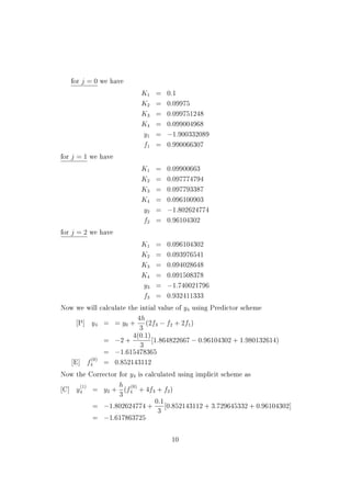
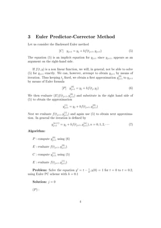
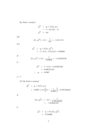
1. The document describes predictor-corrector methods for numerically solving ordinary and partial differential equations. 2. Predictor-corrector methods use an explicit method to predict the next value, then apply an implicit correction method in an iterative process to improve the accuracy of the predicted value. 3. The Euler predictor-corrector method is presented as a basic example, using Euler's explicit method for the predictor and the backward Euler implicit method for the corrector.

1. Numerical solution of ordinary and
partial dierential Equations
Module 16: Predictor-Corrector methods
Dr.rer.nat. Narni Nageswara Rao
£
August 2011
1 General Multistep Methods
Consider the linear multistep methods
yj+1 =
kX
i=0
aiyj i + h
kX
i=0
bifj i + hb 1fj+1j = k; k + 1; ¡¡¡ (1)
Which are k+1 step methods, k ! 0. For k = 0, we recover one-step methods.
The coecients ai, bi are real and fully identify the scheme, thus are such
that ak T= 0, or bk T= 0. If b 1 T= 0 the scheme is implicit, otherwise it is
explicit.
2 Predictor-Corrector Methods
When solving nonlinear IVP of the form
y
H = f(t; y); y(t0) = y0
at each time step implicit schemes require solving nonlinear algebraic equa-
tions. For instance, if the Crack-Nicolson method is used, we get the nonlin-
ear equation
yj+1 = yj +
h
2
[fj + fj+1] = (yj+1)
£nnrao maths@yahoo.co.in
1

2. that can be cast in the form (yj+1) = 0, where (yj+1) = yj+1 (yj+1).
To solve this equation the Newton method would give
y
(n+1)
j+1 = y
(n)
j+1 (y
(n)
j+1)
H(y
(n)
j+1)
for n = 0; 1; ¡¡¡ until convergence and require an initial datum y
(0)
j+1 su-
ciently close to yj+1. Alternatively one can resort to

3. xed point iterations
y
(n+1)
j+1 = (y
(n)
j+1) (2)
for n = 0; 1; ¡¡¡ until convergence. In such a case, the global convergence con-
dition for the

4. xed-point method (see theorem in

5. rst year B-Tech content)
sets a constraint on the diccretization step size of the form
h
1
jb 1jL
(3)
where L is the Lipschitz constant of f with respect to y. In practice, ex-
cept for the case of shift problems, this restriction on h is not signi

6. cant
since considerations of accuracy put a much more restrictive constraint on h.
However, each iteration of (2) requires one evaluation of the function f and
the computational cost can be reduced by providing a good initial guess y
(0)
j+1.
This can be done by taking one step of an explicit multistep method and then
iterating on (2) for a

7. xed numbe m of interations. By doing so, the implicit
multistep method that is employed in the

8. xed-point scheme Corrects the
value of yj+1 predicted by the explicit multistep method. A procedure of
this sort is called a predictor-corrector method. or PC method. There are
many ways in which a predictor-corrector method can be implemented.
2.1 Basic Version
The value y
(0)
j+1 is computed by an explicit ~k + 1-step method called the
Predictor (here identi

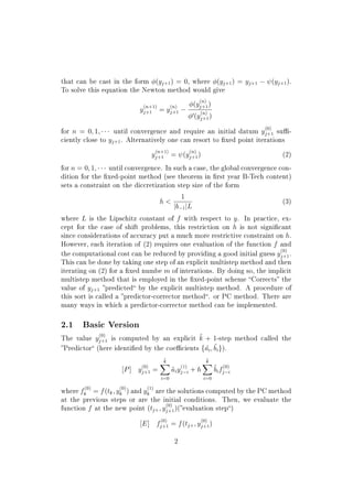
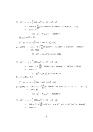
9. ed by the coecients f~ai; ~big).
[P ] y
(0)
j+1 =
~kX
i=0
~aiy
(1)
j i + h
~kX
i=0
~bif
(0)
j i
where f
(0)
k = f(tk; y
(0)
k ) and y
(1)
k are the solutions computed by the PC method
at the previous steps or are the initial conditions. Then, we evaluate the
function f at the new point (tj+; y
(0)
j+1)(evaluation step)
[E] f
(0)
j+1 = f(tj+; y
(0)
j+1)
2

10. and