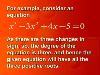
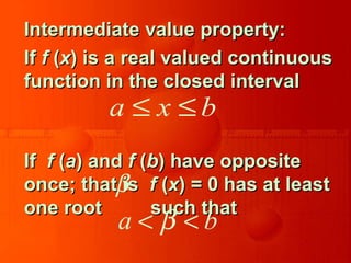
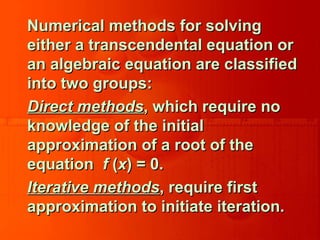
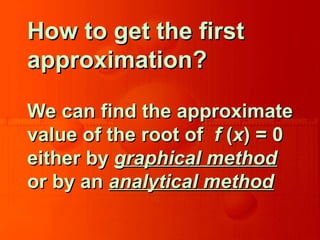
Downloaded 176 times
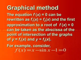
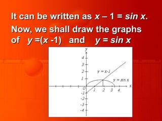
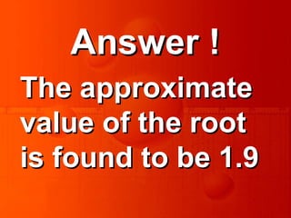
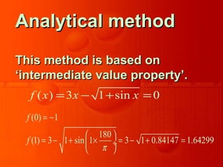


This document discusses various numerical methods for solving non-linear equations, emphasizing techniques such as the bisection method, regula-falsi method, Newton-Raphson method, and others. It explains the classification of equations into algebraic and transcendental, describes properties and roots of algebraic equations, and outlines the conditions for the existence of roots. The document also highlights graphical and analytical methods for obtaining initial approximations of roots.