MATHEMATICS-I
CONTENTS
   Ordinary Differential Equations of First Order and First Degree
   Linear Differential Equations of Second and Higher Order
   Mean Value Theorems
   Functions of Several Variables
   Curvature, Evolutes and Envelopes
   Curve Tracing
   Applications of Integration
   Multiple Integrals
   Series and Sequences
   Vector Differentiation and Vector Operators
   Vector Integration
   Vector Integral Theorems
   Laplace transforms
TEXT BOOKS
   A text book of Engineering Mathematics, Vol-I
    T.K.V.Iyengar, B.Krishna Gandhi and Others,
    S.Chand & Company
   A text book of Engineering Mathematics,
    C.Sankaraiah, V.G.S.Book Links
   A text book of Engineering Mathematics, Shahnaz A
    Bathul, Right Publishers
   A text book of Engineering Mathematics,
    P.Nageshwara Rao, Y.Narasimhulu & N.Prabhakar
    Rao, Deepthi Publications
REFERENCES
 A text book of Engineering Mathematics,
  B.V.Raman, Tata Mc Graw Hill
 Advanced Engineering Mathematics, Irvin
  Kreyszig, Wiley India Pvt. Ltd.
 A text Book of Engineering Mathematics,
  Thamson Book collection
UNIT-III
 CHAPTER-I:MEAN VALUE
      THEOREMS
CHAPTER-II:FUNCTIONS OF
  SEVERAL VARIABLES
UNIT HEADER
  Name of the Course: B.Tech
      Code No:07A1BS02
      Year/Branch: I Year
CSE,IT,ECE,EEE,ME,CIVIL,AERO
         Unit No: III
        No. of slides:17
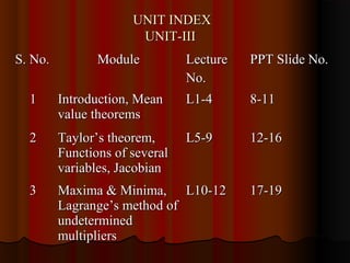
UNIT INDEX
                       UNIT-III
S. No.          Module          Lecture   PPT Slide No.
                                No.
  1      Introduction, Mean     L1-4      8-11
         value theorems
  2      Taylor’s theorem,      L5-9      12-16
         Functions of several
         variables, Jacobian
  3      Maxima & Minima, L10-12          17-19
         Lagrange’s method of
         undetermined
         multipliers
Lecture-1
             INTRODUCTION
 Here we study about Mean value theorems.
 Continuous function: If limit of f(x) as x tends
  c is f(c) then the function f(x) is known as
  continuous function. Otherwise the function is
  known as discontinuous function.
 Example: If f(x) is a polynomial function then
  it is continuous.
Lecture-2
ROLLE’S MEAN VALUE THEOREM
 Let f(x) be a function such that

1) it is continuous in closed interval [a, b];
2) it is differentiable in open interval (a, b) and
3) f(a)=f(b)
Then there exists at least one point c in open
  interval (a, b) such that f '(c)=0
 Example: f(x)=(x+2)3(x-3)4 in [-2,3]. Here c=-
  2 or 3 or 1/7
Lecture-3
     LAGRANGE’S MEAN VALUE
           THEOREM
 Let f(x) be a function such that

1) it is continuous in closed interval [a, b] and
2) it is differentiable in open interval (a, b)
Then there exists at least one point c in open
  interval (a, b) such that f '(c)=[f(b)-f(a)]/[b-a]
 Example: f(x)=x3-x2-5x+3 in [0,4]. Here
  c=1+√37/3
Lecture-4
       CAUCHY’S MEAN VALUE
            THEOREM
 If f:[a, b] →R, g:[a, b] →R are such that
  1)f,g are continuous on [a, b]
  2)f,g are differentiable on (a, b) and
  3)g '(x)≠0 for all xЄ(a, b) then there exists
  cЄ(a, b) such that
  [f(b)-f(a)]/[g(b)-g(a)]=f ′(c)/g′(c)
 Example: f(x)=√x, g(x)=1/√x in [a,b]. Here
  c=√ab
Lecture-5
          TAYLOR’S THEOREM
 If f:[a, b]→R is such that
  1)f (n-1) is continuous on [a, b]            2)f(n-1)
  is derivable on (a, b) then there exists a point
  cЄ(a, b) such that                     f(b)=f(a)+
  (b-a)/1!f '(a)+(b-a)2/2!f "(a)+…..
 Example: f(x)=ex. Here Taylor’s expansion at
  x=0 is 1+x+x2/2!+…..
Lecture-6
       MACLAURIN’S THEOREM
 If f:[0,x]→R is such that
  1)f(n-1) is continuous on [0,x]
  2)f(n-1) is derivable on (0,x) then there exists a
  real number θЄ(0,1) such that
  f(x)=f(0) + xf '(0) +x2/2! f "(0) +………
 Example: f(x)=Cosx. Here Maclaurin’s
  expansion is 1-x2/2!+x4/4!-….
Lecture-7
       FUNCTIONS OF SEVERAL
            VARIABLES
 We have already studied the notion of limit,
  continuity and differentiation in relation of
  functions of a single variable. In this chapter
  we introduce the notion of a function of
  several variables i.e., function of two or more
  variables.
 Example 1: Area A= ab
 Example 2: Volume V= abh
Lecture-8
                    DEFINITIONS
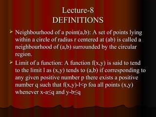
   Neighbourhood of a point(a,b): A set of points lying
    within a circle of radius r centered at (ab) is called a
    neighbourhood of (a,b) surrounded by the circular
    region.
   Limit of a function: A function f(x,y) is said to tend
    to the limit l as (x,y) tends to (a,b) if corresponding to
    any given positive number p there exists a positive
    number q such that f(x,y)-l<p foa all points (x,y)
    whenever x-a≤q and y-b≤q
Lecture-9
                 JACOBIAN
 Let u=u(x,y), v=v(x,y). Then these two
  simultaneous relations constitute a
  transformation from (x,y) to (u,v). Jacobian of
  u,v w.r.t x,y is denoted by J[u,v]/[x,y] or
  ∂(u,v)/∂(x,y)
 Example: x=r cosθ,y=r sinθ then ∂(x,y)/∂(r,θ)
  is r and ∂(r,θ)/∂(x,y)=1/r
Lecture-10
  MAXIMUM AND MINIMUM OF
 FUNCTIONS OF TWO VARIABLES
 Let f(x,y) be a function of two variables x and
  y. At x=a, y=b, f(x,y) is said to have maximum
  or minimum value, if f(a,b)>f(a+h,b+k) or
  f(a,b)<f(a+h,b+k) respectively where h and k
  are small values.
 Example: The maximum value of
  f(x,y)=x3+3xy2-3y2+4 is 36 and minimum value
  is -36
Lecture-11
             EXTREME VALUE
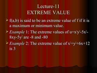
 f(a,b) is said to be an extreme value of f if it is
  a maximum or minimum value.
 Example 1: The extreme values of u=x2y2-5x2-
  8xy-5y2 are -8 and -80
 Example 2: The extreme value of x2+y2+6x+12
  is 3
Lecture-12
      LAGRANGE’S METHOD OF
    UNDETERMINED MULTIPLIERS
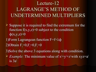
 Suppose it is required to find the extremum for the
  function f(x,y,z)=0 subject to the condition
  ф(x,y,z)=0
1)Form Lagrangean function F=f+λф
2)Obtain Fx=0,Fy=0,Fz=0
3)Solve the above 3 equations along with condition.
 Example: The minimum value of x2+y2+z2 with xyz=a3
  is 3a2

M1 unit iii-jntuworld

  • 1.
  • 2.
    CONTENTS  Ordinary Differential Equations of First Order and First Degree  Linear Differential Equations of Second and Higher Order  Mean Value Theorems  Functions of Several Variables  Curvature, Evolutes and Envelopes  Curve Tracing  Applications of Integration  Multiple Integrals  Series and Sequences  Vector Differentiation and Vector Operators  Vector Integration  Vector Integral Theorems  Laplace transforms
  • 3.
    TEXT BOOKS  A text book of Engineering Mathematics, Vol-I T.K.V.Iyengar, B.Krishna Gandhi and Others, S.Chand & Company  A text book of Engineering Mathematics, C.Sankaraiah, V.G.S.Book Links  A text book of Engineering Mathematics, Shahnaz A Bathul, Right Publishers  A text book of Engineering Mathematics, P.Nageshwara Rao, Y.Narasimhulu & N.Prabhakar Rao, Deepthi Publications
  • 4.
    REFERENCES  A textbook of Engineering Mathematics, B.V.Raman, Tata Mc Graw Hill  Advanced Engineering Mathematics, Irvin Kreyszig, Wiley India Pvt. Ltd.  A text Book of Engineering Mathematics, Thamson Book collection
  • 5.
    UNIT-III CHAPTER-I:MEAN VALUE THEOREMS CHAPTER-II:FUNCTIONS OF SEVERAL VARIABLES
  • 6.
    UNIT HEADER Name of the Course: B.Tech Code No:07A1BS02 Year/Branch: I Year CSE,IT,ECE,EEE,ME,CIVIL,AERO Unit No: III No. of slides:17
  • 7.
    UNIT INDEX UNIT-III S. No. Module Lecture PPT Slide No. No. 1 Introduction, Mean L1-4 8-11 value theorems 2 Taylor’s theorem, L5-9 12-16 Functions of several variables, Jacobian 3 Maxima & Minima, L10-12 17-19 Lagrange’s method of undetermined multipliers
  • 8.
    Lecture-1 INTRODUCTION  Here we study about Mean value theorems.  Continuous function: If limit of f(x) as x tends c is f(c) then the function f(x) is known as continuous function. Otherwise the function is known as discontinuous function.  Example: If f(x) is a polynomial function then it is continuous.
  • 9.
    Lecture-2 ROLLE’S MEAN VALUETHEOREM  Let f(x) be a function such that 1) it is continuous in closed interval [a, b]; 2) it is differentiable in open interval (a, b) and 3) f(a)=f(b) Then there exists at least one point c in open interval (a, b) such that f '(c)=0  Example: f(x)=(x+2)3(x-3)4 in [-2,3]. Here c=- 2 or 3 or 1/7
  • 10.
    Lecture-3 LAGRANGE’S MEAN VALUE THEOREM  Let f(x) be a function such that 1) it is continuous in closed interval [a, b] and 2) it is differentiable in open interval (a, b) Then there exists at least one point c in open interval (a, b) such that f '(c)=[f(b)-f(a)]/[b-a]  Example: f(x)=x3-x2-5x+3 in [0,4]. Here c=1+√37/3
  • 11.
    Lecture-4 CAUCHY’S MEAN VALUE THEOREM  If f:[a, b] →R, g:[a, b] →R are such that 1)f,g are continuous on [a, b] 2)f,g are differentiable on (a, b) and 3)g '(x)≠0 for all xЄ(a, b) then there exists cЄ(a, b) such that [f(b)-f(a)]/[g(b)-g(a)]=f ′(c)/g′(c)  Example: f(x)=√x, g(x)=1/√x in [a,b]. Here c=√ab
  • 12.
    Lecture-5 TAYLOR’S THEOREM  If f:[a, b]→R is such that 1)f (n-1) is continuous on [a, b] 2)f(n-1) is derivable on (a, b) then there exists a point cЄ(a, b) such that f(b)=f(a)+ (b-a)/1!f '(a)+(b-a)2/2!f "(a)+…..  Example: f(x)=ex. Here Taylor’s expansion at x=0 is 1+x+x2/2!+…..
  • 13.
    Lecture-6 MACLAURIN’S THEOREM  If f:[0,x]→R is such that 1)f(n-1) is continuous on [0,x] 2)f(n-1) is derivable on (0,x) then there exists a real number θЄ(0,1) such that f(x)=f(0) + xf '(0) +x2/2! f "(0) +………  Example: f(x)=Cosx. Here Maclaurin’s expansion is 1-x2/2!+x4/4!-….
  • 14.
    Lecture-7 FUNCTIONS OF SEVERAL VARIABLES  We have already studied the notion of limit, continuity and differentiation in relation of functions of a single variable. In this chapter we introduce the notion of a function of several variables i.e., function of two or more variables.  Example 1: Area A= ab  Example 2: Volume V= abh
  • 15.
    Lecture-8 DEFINITIONS  Neighbourhood of a point(a,b): A set of points lying within a circle of radius r centered at (ab) is called a neighbourhood of (a,b) surrounded by the circular region.  Limit of a function: A function f(x,y) is said to tend to the limit l as (x,y) tends to (a,b) if corresponding to any given positive number p there exists a positive number q such that f(x,y)-l<p foa all points (x,y) whenever x-a≤q and y-b≤q
  • 16.
    Lecture-9 JACOBIAN  Let u=u(x,y), v=v(x,y). Then these two simultaneous relations constitute a transformation from (x,y) to (u,v). Jacobian of u,v w.r.t x,y is denoted by J[u,v]/[x,y] or ∂(u,v)/∂(x,y)  Example: x=r cosθ,y=r sinθ then ∂(x,y)/∂(r,θ) is r and ∂(r,θ)/∂(x,y)=1/r
  • 17.
    Lecture-10 MAXIMUMAND MINIMUM OF FUNCTIONS OF TWO VARIABLES  Let f(x,y) be a function of two variables x and y. At x=a, y=b, f(x,y) is said to have maximum or minimum value, if f(a,b)>f(a+h,b+k) or f(a,b)<f(a+h,b+k) respectively where h and k are small values.  Example: The maximum value of f(x,y)=x3+3xy2-3y2+4 is 36 and minimum value is -36
  • 18.
    Lecture-11 EXTREME VALUE  f(a,b) is said to be an extreme value of f if it is a maximum or minimum value.  Example 1: The extreme values of u=x2y2-5x2- 8xy-5y2 are -8 and -80  Example 2: The extreme value of x2+y2+6x+12 is 3
  • 19.
    Lecture-12 LAGRANGE’S METHOD OF UNDETERMINED MULTIPLIERS  Suppose it is required to find the extremum for the function f(x,y,z)=0 subject to the condition ф(x,y,z)=0 1)Form Lagrangean function F=f+λф 2)Obtain Fx=0,Fy=0,Fz=0 3)Solve the above 3 equations along with condition.  Example: The minimum value of x2+y2+z2 with xyz=a3 is 3a2