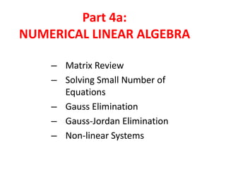
Part 4a:
NUMERICAL LINEAR ALGEBRA
– Matrix Review
– Solving Small Number of
Equations
– Gauss Elimination
– Gauss-Jordan Elimination
– Non-linear Systems
Matrix Notation:

a11
a21
..

A

a12 .. a1m
..
..

an1

..

.. anm

row

nxm

column

mx1
1xn
m=n

a column vector
a row vector
symmetric matrix

Addition/subtraction of two matrices:
C

A

B

cij

aij

bij

(add/subtract corresponding terms)

both A and B must have same sizes.
Multiplication of matrices:
n

C

cij

A B

aik bkj
k 1

A nxm B mxl

C

> First matrix must have the same number of columns as
the number of rows in the second matrix.

nxl

EX: Calculate [X][Y] such that:

3 1
X

8 6
0 4

Y

5 9
7 2

Division of matrices:

I

C

B

1

B

B B

A/B

A B

1

inverse of B: exist only if matrix A is square and
non-singular.
1

İf B-1 exist, division is same as multiplicaton
Transpose:

a11

a31

a21

a22

a23

a31

a32

a33

a11

a21

a31

a21

a22

a23

a31

A

a21

a32

a33

a11

a31

a21

a22

a32

a31

A

T

a21
a23

a33

Trace:

A

tr A

a11 a22

a33

Augmentation:

a11
A

a21

a31

a21

a22

a23

a31

a32

a33

a11
C

a21

a31

b1

a21

a22

a23

b2

a31

a32

a33

b3
Determinant for 2x2 matrix:

a11

A

a12

a11

A

a21 a22

a12

a21 a22

a11a22 a12 a21

Determinant for 3x3 matrix:
a11

a13

a21

a22

a23

a31

A

a12
a32

a33

a11
A

a12

a13

a21

a22

a23

a31

a32

a33

a11

a22

a23

a32

a33

a12

a21

a23

a31

a33

a13

a21

a22

a31

a32
Linear Algebraic Equations in Matrix form:
Consider a system of n linear equations with n unknowns:
a11 x1 a12 x2 ... a1n xn

b1

a21 x1 a22 x2 ... a2 n xn

b2

...
an1 x1 an 2 x2 ... ann xn

a ' s : coefficients
x ' s : unknowns
b' s :

constants

bn

 For small n’s (say, n <= 3) this can be done by hand, but for large
n’s we need computer power ( numerical techniques).
 In engineering, multi-component systems require solution of a set
of mathematical equations that need to be solved simultaneously.

need to define pressure at every point (unknowns), on
the surface, and solve the underlying physical equation
simultenously.
Symbolic form of the linear system
a11 x1 a12 x2 ... a1n xn

b1

a21 x1 a22 x2 ... a2 n xn

b2

...
an1 x1 an 2 x2 ... ann xn

bn

Matrix form of the linear system

a11
A

a12

a21
..
an1

.. a1n
..
..

..

x

.. ann

Ax b

x1
x2
..
xn

b

b1
b2
..
bn
Gauss Elimination
We want to solve
a11 x1 a12 x2 ... a1n xn

b1

a21 x1 a22 x2 ... a2 n xn

b2

...
an1 x1 an 2 x2 ... ann xn

bn

One way to solve it

Ax b

1

A Ax

1

A b

x

1

A b

if the inverse of
A exist!

 Even if an inverse of A exist, this method is computationally not
efficient.
 We have more efficient methods to solve the linear system.
 These solutions do not require operations involving calculating
the inverse of A.
Solving small number of linear equations:
1-Graphical Method:
x2
a11 x1 a12 x2

x2

b2

b1
a12

a21
x1
a22

b1
a22

b1

a21 x1 a22 x2

a11
x1
a12

intersection of
two lines gives
the solution

EX: Use graphical method to solve:

3x1 2 x2
x1 2 x2

18
2

x2
9

3

x2

1
x1 1
2

x2

3
x1 9
2

1
0

4

x1
 For three equations (unknowns: x1 , x2 , x3 ), each equation
represents a plane in a 3-D space. Solution is where three planes
intersect.
 For n>3, graphical method fails.
 It is useful for visualizing the behavior of linear systems.
x2

x2

x2

x1
No solution

x1
Infinite solutions

x1
Ill-conditioned
system
2-Cramer’s Rule:
For the previous example, calculate determinant of coefficients.
3x1 2 x2

18

x1 2 x2

2

3

A

2

3

A

2

1 2

1 2

3 2 ( 1) 2 8

For special cases:
x2

x2

x1
A

0.5 1
0.5 1

0

x1
A

0.5 1
1

2

0

x1
A

0.46 1
0.5

1

0.04

Singular systems have zero determinants; ill-conditioned systems have near-zero
determinants.
 In Cramer’s rule, we replace the column of the coefficients of
the unknown by the column of the constants, and divide by
the determinant, i.e. (for n=3),

x1

b1
b2
b3

a12
a22
a32

a13
a23
a33

A

x2

a11 b1
a21 b2
a31 b3

a13
a23
a33

A

x3

a11
a21
a31

a12
a22
a32

b1
b2
b3

A

EX: Use Cramer’s rule to solve:

0.3x1 0.52 x2
0.5 x1

x3

0.01

x2 1.9 x3

0.67

0.1x1 0.3x2

0.5 x3

0.44

 For n>3, Cramer’s rule also becomes impractical and timeconsuming for calculation of the determinants.
3-Elimination of Unknowns:
a11 x1 a12 x2

b1

a21a11 x1 a21a12 x2

a21b1

a21 x1 a22 x2

b2

a11a21 x1 a11a22 x2

a11b2

subtract first eqn. from the second one to eliminate one of
the unknowns to get:
a11a22 x2

a21a12 x2

a11b2

a21b1

Then, solve for the second unknown
x2

a11b2 a21b1
a11a22 a12 a21

For the first unknown , use either of the original eqn:
x1

a22b1 a12b2
a11a22 a12 a21

EX: Use the elimination of unknowns to solve:
x1 2 x2
3x1 2 x2 18

2
Naive Gauss Elimination:
 We apply the same method of elimination of unknowns to a system
of n equations.
> Eliminate unknowns until reaching a single unknown.
> Back-substitute into the original equation to find other unknowns.
a11 x1 a12 x2 ... a1n xn

b1

a21 x1 a22 x2 ... a2 n xn

b2

...
an1 x1 an 2 x2 ... ann xn

bn

Elimination:
To eliminate (x1 ), multiply the first equation by a21/a11 :
a21 x1

a21
a12 x2 ...
a11

a21
a1n xn
a11

a21
b1
a11

Divison by a11 is also
called “normalization”
subtract this equation from the second one:
a22

or

a21
a12 x2 ...
a11

a12
a1n xn
a11

a2 n

'
'
a22 x2 ... a2 n xn

b2

a12
b1
a11

x1 eliminated

'
b2

Same procedure is applied for the third equation, i.e., multiply the
first equation by a31/a11 and subtract from the third equation. This
will eliminate (x1) from the third equation.
a11 x1 a12 x2

b1

'
a22 x2

pivot
element

a13 x3 ... a1n xn
'
'
a23 x3 ... a2 n xn

'
b2

'
a32 x2

'
'
a33 x3 ... a3n xn

b3'

'
'
an 3 x3 ... ann xn

'
b2

...
'
a n 2 x2

pivot
equation

x1 eliminated
from all
equations
except the
first one.
Elimination of the second unknown (x2):
a11 x1 a12 x2

b1

'
'
a23 x3 ... a2 n xn

'
b2

''
'
a33 x3 ... a3' n xn

'
a22 x2

a13 x3 ... a1n xn

'
b3'

x2 eliminated
from all
equations
except the
first and
second one.

...
'
''
an' 3 x3 ... ann xn

'
b2'

The process can be repeated for all other unknowns to get an
upper-triangular system:
a11 x1 a12 x2
'
a22 x2

a13 x3 ... a1n xn

b1

'
'
a23 x3 ... a2 n xn

'
b2

''
'
a33 x3 ... a3' n xn

'
b3'

...
(n
ann 1) xn

(
bnn

1)

indicates the
number of
operations
performed until the
upper triangular
system forms.
Back-substitution:
Solve for (xn) simply by:
xn

(
bnn
n
a (nn

1)
1)

Value of xn can be back-substituted into the upper equation in
upper triangular system to solve for (xn-1). The procedure is
repeated for all remaining unknowns.
n
( i 1)
i

(
aiji 1) x j

b
xi

j i 1
( i 1)

for i

n 1, n 2, ... , 1

a ii

EX: Use Gauss elimination to solve (carrying 6 S.D.’s):
3x1 0.1x2

0.2 x3

0.1x1 7 x2

0.3x3

0.3x1 0.2 x2 10 x3

7.85
19 .3
71 .4
Operation Counting:
 The time of execution in the elimination/back-substitution
processes depends on the total number of addition/subtraction
and multiplication/division operations (combined called as
floating point operations- FLOPs).
 Total number of FLOPs for the solution of a system size n using
Gauss elimination can be counted from the algorithm.
n

Elimination

Back-substitution Total FLOPS

10

375

55

430

100

338250

5050

343300

1000

3.34E+08

500500

3.34E+08

FLOPs for Gauss Elimination

n3/3 + O(n2)

 Most of the FLOPS are due to the elimination stage.
Pitfalls of the elimination:
 The following topics concerns all elimination techniques as well as
Gauss elimination.
Divison by Zero:
 In naive Gauss elimination, if one of the coefficients is zero, a
division-by-zero occurs during normalization.
 If the coefficient is nearly zero problems still arise (due to roundoff errors).
 Pivoting (discussed later) will provide a partial remedy.
Round-off errors:
 Due to limited amount of S.F. in computer numbers, a round-off
error in the results will always occur.
 They can be important when large number of operations (>100)
involved.
 Using more significant figures (double precision) lead to lower
round-off errors.
Ill-conditioned systems:
 Small changes in the coefficients results in large changes in the
solution (ill-conditioned system).
 In a different approach a wide range of solutions approximately
satisfy the equations.
 In these systems, small changes in the coefficients due to roundoff errors lead to large errors in solution.
 In these systems, numerical approximations lead to larger errors.
EX: a) Solve
x1 2 x2 10
1.1x1 2 x2

10 .4

b) Now solve
x1 2 x2 10
1.05 x1 2 x2

10 .4

c) Compute the determimnants

A small change in the
coefficient results in
very different
solutions.
Near-zero
determinants of the
system indicate illconditoning.
 It is difficult to detemine how close to zero a determinant
indicates ill-conditioning. This is due to the fact that magnitude of
the determinant can be changed by scaling the equation even
though the solution does not change.
EX: Compare determinants for
a)

b)

c)

3x1 2 x2

18

x1 2 x2

scale equations such
that the maximum
coefficient for each
row is 1.

2

x1 2 x2 10
1.1x1 2 x2 10 .4
10 x1 20 x2

100

11x1 20 x2

104

x10

EX: Scale the systems of equations
in the previous example and
recompute the determinants.
Determinant
(after scaling)

System
condition

 How can we calculate determinant for large systems?
 Gauss elimination has the extra bonus of calculating the
determinant:
Determinant of a triangular matrix can simply be computed
as the product of its diagonal elements.
a11 x1 a12 x2

b1

'
'
a23 x3 ... a2 n xn

'
b2

''
'
a33 x3 ... a3' n xn

'
a22 x2

a13 x3 ... a1n xn

'
b3'

...
(n
ann 1) xn

D

'
''
11 22 33

a a a ...a

( n 1)
nn

( 1)

p

(
b2n

1)

p= number of times pivoting
applied (discussed later)
Singular systems:
 This is the worse case of ill-conditioning where two or more
equations are identical.
 In this case, system loose a degree of freedom which makes
solution impossible a singular system.
 In large systems, it may not be easy to see that the system is
singular. We can detect singularity by calculating the
determinant.

If D=0

Singular system

 In Gauss elimination, this means a “zero” is encountered in
diagonal elements.
 If a zero is encountered during elimination terminate the
calculation.
Improvements on the elimination:
 So far we mentioned the possible problems in naive Gauss
elimination; here we discuss some solutions of these
problems.
Pivoting:
 If pivot=0, a divison-by-zero occurs during normalization.
 As remedy (partial pivoting),

Find the element below the pivot column whose absolute
value is the largest.
Switch the pivot row with row of the the largest element.
 If both rows and columns are searched for the largest
element complete pivoting (not a common practice)
 Pivoting is in general adventegous to reduce round-off errors
during the elimination even if the pivot element is not zero.
 By these adventages, pivoting is routinely applied in Gauss
elimination.
EX: Use Gauss elimination to solve the system
0.0003 x1 3.0000 x2
1.0000 x1 1.0000 x2

0

Exact solution
x1=0.3333.. ;
x2=0.6666..

2.0001
1.0000

a) Naive elimination (multiply the first eqn by 1/0.0003 and subtract to yield)
0.0003 x1 3.0000 x2

2.0001

9999 x2

6666

Back-substition:

x2

0.6666 ..

b) Now apply pivoting
1.0000 x1 1.0000 x2 1.0000
0.0003 x1 3.0000 x2 2.0001

Elimination
1.0000 x1 1.0000 x2 1.0000
2.9997 x2 1.9998

x1

x2

3

0.667

-3.33

4

0.6667

0.0000

5

x1

2.0001 3(2 / 3)
0.0003

S.F.

0.66667

0.30000

6

0.666667

0.330000

7

0.6666667

0.3330000

x2

0.6666 ..

back-substition:
x1 0.3333 ..

Note that the
system is not illconditioned.
Scaling:
 In engineering applications, equations with widely differents
units may have to be solved simultenously, e.g.,
.. .. x1..m (millivolts)
)
.. .. xm 1..n (kilovolts

..
..

 This may result in large variations in the coefficients and
constants.
 This results in large round-off errors during elimination.
EX: Use Gauss elimination to solve the system (using 3 significant figures):
Exact solution:
x1=1.00002
x2=0.99998

2 x1 100 ,000 x2 100 ,000
x1 x2 2

note the scale problem!

a) Elimination with pivoting (without scaling):
2 x1 100 ,000 x2
elimination

50 ,000 x2

100 ,000
50 ,000

b-substitution

x2

1.00

x1

0.00 (100% error)
b) Repeat with scaling (i.e. divide each raw by the largest coefficient):
0.00002 x1 x2 1
x1 x2 2
pivoting
scaling
x1 x2 2
0.00002 x1 x2 1
x1
elimination

x2
x2

2

b-substitution

1.00

x2 1
x1 1

Scaling result in
the correct result
(for 3 S.F.)

c) Now, apply scaling for just pivoting (keep original eqn’s):
pivoting

b-substitution

x1

x2

2 x1 100 ,000 x2
x2 1
x1 1

2
100 ,000

elimination

x1

x2

100 ,000 x2

2
100 ,000

We used scaling just to determine whether pivoting was
necessary.
Eqn’s did not require scaling to arrive the correct result.

 Since scaling introduces extra round-off errors, we apply scaling
only as a criterion for pivoting.
 If determinant is not needed (which is the case most of the
time), the strategy is scale for just pivoting, but use the original
coefficients for the elimination and back-substitution.
Gauss-Jordan Elimination:
 In this method, unknowns are eliminated from all the raws; not just
from the subsequent ones. So, instead of an upper triangular
matrix, one gets a diagonal matrix.
 In addition, all raws are normalized by dividining them to the pivot
element. So, the final matrix is an identity matrix.
Gauss Elimination
a11 x1 a12 x2

Gauss-Jordan Elimination
b1

'
'
a23 x3 ... a2 n xn

'
b2

''
'
a33 x3 ... a3' n xn

'
a22 x2

a13 x3 ... a1n xn

b1( n )

b3''

x1

...
a

(
b2 n )

x2
x3

b3( n )

...

( n 1)
nn
n

x

( n 1)
n

b

 It is not necessary to apply back-substitution!

...
xn

shows total number
of operations applied

(n
bn )
EX: Gauss-Jordan technique to solve the system of equations (6 S.D.):
3x1 0.1x2

0.2 x3

0.1x1 7 x2

0.3x3

0.3x1 0.2 x2 10 x3

7.85
19 .3
71 .4

First, form an augmented system:

3

0.1

0.2

0 .1

7

0.3

0. 3

0.2

10

7.85
19.3
71.4

Normalize the first raw:

1

0.0333333

0.066667 2.61667

0. 1

7

0.3

0.3

0.2

10

19.3
71.4
Eliminate x1 term from the second and third raws:

1

0.0333333

0.066667

2.61667

0

7.00333

0.293333

19.5617

0

0.190000

10.0200

70.6150

Normalize the second raw

1

0.0333333

0
0

1
0.190000

0.066667
0.0418848
10.0200

2.61667
2.79320
70.6150

Eliminate x2 term from the first and third raws:

1 0

0.0680629

0 1

0.0418848

0 0

10.01200

2.52356
2.79320
70.0843
Normalize the third raw:

1 0

0.0680629

0 1

0.0418848

0 0

1

2.52356
2.79320
7.00003

Finally, eliminate x3 term from the first and second raws:

1 0 0
0 1 0
0 0 1

3.00000
2.50001
7.00003

x1
x2

3.00000
2.50001

x3

7.00003

 The same pivoting strategy as in Gauss elimination can be applied.
 Number of processes (FLOPs) is slightly larger than Gauss
elimination.
FLOPS for Gauss-Jordan

n3/2 + O(n2)

about 50% more
operations in G-J
Working with Complex Variables:
 In some cases, we may have to face with complex variables in the
system of equations.
C Z

W

where
C

A

iB

Z

X

iY

W

U

iV

 If the language you are using supports complex variables (such as
Fortran, Matlab), then you don’t need to do anything.
 Alternatively, the complex system can be rewritten by substituting
the real and imaginary parts, and equating real and imaginary parts
separately. Thus,
A X

B Y

U

A

B X

A Y

V

B

B X
A

Y

U
V

instead of an nxn
complex
system, we have
a 2nx2n real
system
Nonlinear System of Equations:
 Consider a system of n non-linear equations with n unknowns:
f1 ( x1 , x2 ,..., xn )

0

f 2 ( x1 , x2 ,..., xn )

0

...
f n ( x1 , x2 ,..., xn )

0

 In the previous chapter, we developed a solution method for a
system of n=2 (multi-equation Newton-Raphson method).
 In order to evaluate the problem as a linear system, we can expand
the equations using first-order Taylor series expansion, i.e., for k-th
row
f k ,i

1

set to zero

f k ,i

( x1,i

1

x1,i )

f k ,i
x1

unknowns

( x2 ,i

1

x2 ,i )

f k ,i
x2

... ( xn ,i

1

xn ,i )

f k ,i
xn
re-arranging the terms
( x1,i 1 )

f k ,i
x1

f k ,i

( x2 ,i 1 )

x2

... ( xn ,i 1 )

f k ,i
xn

f k ,i

x1,i

f k ,i
x1

x2 ,i

f k ,i
x2

... xn ,i

Define matrices
f1,i
x1
f 2 ,i

x2
f 2 ,i

x1
...
f n ,i

x2
...
f n ,i

x1

Z

f1,i

x2

...
...
...
...

f1,i
xn
f 2 ,i
xn
...
f n ,i

Xi

1

x1,i 1
x2 ,i 1
...
x n ,i 1

Fi

...
f n ,i

Xi

x1,i
x 2 ,i
...
x n ,i

xn

Then,
Z Xi

f1,i
f 2 ,i

1

Fi

Z Xi

Note that the solution is reached iteratively.

This equation is in the
form of Ax=b, and can
be solved using Gauss
elimination

f k ,i
xn

Es272 ch4a

  • 1.
    Part 4a: NUMERICAL LINEARALGEBRA – Matrix Review – Solving Small Number of Equations – Gauss Elimination – Gauss-Jordan Elimination – Non-linear Systems
  • 2.
    Matrix Notation: a11 a21 .. A a12 ..a1m .. .. an1 .. .. anm row nxm column mx1 1xn m=n a column vector a row vector symmetric matrix Addition/subtraction of two matrices: C A B cij aij bij (add/subtract corresponding terms) both A and B must have same sizes.
  • 3.
    Multiplication of matrices: n C cij AB aik bkj k 1 A nxm B mxl C > First matrix must have the same number of columns as the number of rows in the second matrix. nxl EX: Calculate [X][Y] such that: 3 1 X 8 6 0 4 Y 5 9 7 2 Division of matrices: I C B 1 B B B A/B A B 1 inverse of B: exist only if matrix A is square and non-singular. 1 İf B-1 exist, division is same as multiplicaton
  • 4.
  • 5.
    Determinant for 2x2matrix: a11 A a12 a11 A a21 a22 a12 a21 a22 a11a22 a12 a21 Determinant for 3x3 matrix: a11 a13 a21 a22 a23 a31 A a12 a32 a33 a11 A a12 a13 a21 a22 a23 a31 a32 a33 a11 a22 a23 a32 a33 a12 a21 a23 a31 a33 a13 a21 a22 a31 a32
  • 6.
    Linear Algebraic Equationsin Matrix form: Consider a system of n linear equations with n unknowns: a11 x1 a12 x2 ... a1n xn b1 a21 x1 a22 x2 ... a2 n xn b2 ... an1 x1 an 2 x2 ... ann xn a ' s : coefficients x ' s : unknowns b' s : constants bn  For small n’s (say, n <= 3) this can be done by hand, but for large n’s we need computer power ( numerical techniques).  In engineering, multi-component systems require solution of a set of mathematical equations that need to be solved simultaneously. need to define pressure at every point (unknowns), on the surface, and solve the underlying physical equation simultenously.
  • 7.
    Symbolic form ofthe linear system a11 x1 a12 x2 ... a1n xn b1 a21 x1 a22 x2 ... a2 n xn b2 ... an1 x1 an 2 x2 ... ann xn bn Matrix form of the linear system a11 A a12 a21 .. an1 .. a1n .. .. .. x .. ann Ax b x1 x2 .. xn b b1 b2 .. bn
  • 8.
    Gauss Elimination We wantto solve a11 x1 a12 x2 ... a1n xn b1 a21 x1 a22 x2 ... a2 n xn b2 ... an1 x1 an 2 x2 ... ann xn bn One way to solve it Ax b 1 A Ax 1 A b x 1 A b if the inverse of A exist!  Even if an inverse of A exist, this method is computationally not efficient.  We have more efficient methods to solve the linear system.  These solutions do not require operations involving calculating the inverse of A.
  • 9.
    Solving small numberof linear equations: 1-Graphical Method: x2 a11 x1 a12 x2 x2 b2 b1 a12 a21 x1 a22 b1 a22 b1 a21 x1 a22 x2 a11 x1 a12 intersection of two lines gives the solution EX: Use graphical method to solve: 3x1 2 x2 x1 2 x2 18 2 x2 9 3 x2 1 x1 1 2 x2 3 x1 9 2 1 0 4 x1
  • 10.
     For threeequations (unknowns: x1 , x2 , x3 ), each equation represents a plane in a 3-D space. Solution is where three planes intersect.  For n>3, graphical method fails.  It is useful for visualizing the behavior of linear systems. x2 x2 x2 x1 No solution x1 Infinite solutions x1 Ill-conditioned system
  • 11.
    2-Cramer’s Rule: For theprevious example, calculate determinant of coefficients. 3x1 2 x2 18 x1 2 x2 2 3 A 2 3 A 2 1 2 1 2 3 2 ( 1) 2 8 For special cases: x2 x2 x1 A 0.5 1 0.5 1 0 x1 A 0.5 1 1 2 0 x1 A 0.46 1 0.5 1 0.04 Singular systems have zero determinants; ill-conditioned systems have near-zero determinants.
  • 12.
     In Cramer’srule, we replace the column of the coefficients of the unknown by the column of the constants, and divide by the determinant, i.e. (for n=3), x1 b1 b2 b3 a12 a22 a32 a13 a23 a33 A x2 a11 b1 a21 b2 a31 b3 a13 a23 a33 A x3 a11 a21 a31 a12 a22 a32 b1 b2 b3 A EX: Use Cramer’s rule to solve: 0.3x1 0.52 x2 0.5 x1 x3 0.01 x2 1.9 x3 0.67 0.1x1 0.3x2 0.5 x3 0.44  For n>3, Cramer’s rule also becomes impractical and timeconsuming for calculation of the determinants.
  • 13.
    3-Elimination of Unknowns: a11x1 a12 x2 b1 a21a11 x1 a21a12 x2 a21b1 a21 x1 a22 x2 b2 a11a21 x1 a11a22 x2 a11b2 subtract first eqn. from the second one to eliminate one of the unknowns to get: a11a22 x2 a21a12 x2 a11b2 a21b1 Then, solve for the second unknown x2 a11b2 a21b1 a11a22 a12 a21 For the first unknown , use either of the original eqn: x1 a22b1 a12b2 a11a22 a12 a21 EX: Use the elimination of unknowns to solve: x1 2 x2 3x1 2 x2 18 2
  • 14.
    Naive Gauss Elimination: We apply the same method of elimination of unknowns to a system of n equations. > Eliminate unknowns until reaching a single unknown. > Back-substitute into the original equation to find other unknowns. a11 x1 a12 x2 ... a1n xn b1 a21 x1 a22 x2 ... a2 n xn b2 ... an1 x1 an 2 x2 ... ann xn bn Elimination: To eliminate (x1 ), multiply the first equation by a21/a11 : a21 x1 a21 a12 x2 ... a11 a21 a1n xn a11 a21 b1 a11 Divison by a11 is also called “normalization”
  • 15.
    subtract this equationfrom the second one: a22 or a21 a12 x2 ... a11 a12 a1n xn a11 a2 n ' ' a22 x2 ... a2 n xn b2 a12 b1 a11 x1 eliminated ' b2 Same procedure is applied for the third equation, i.e., multiply the first equation by a31/a11 and subtract from the third equation. This will eliminate (x1) from the third equation. a11 x1 a12 x2 b1 ' a22 x2 pivot element a13 x3 ... a1n xn ' ' a23 x3 ... a2 n xn ' b2 ' a32 x2 ' ' a33 x3 ... a3n xn b3' ' ' an 3 x3 ... ann xn ' b2 ... ' a n 2 x2 pivot equation x1 eliminated from all equations except the first one.
  • 16.
    Elimination of thesecond unknown (x2): a11 x1 a12 x2 b1 ' ' a23 x3 ... a2 n xn ' b2 '' ' a33 x3 ... a3' n xn ' a22 x2 a13 x3 ... a1n xn ' b3' x2 eliminated from all equations except the first and second one. ... ' '' an' 3 x3 ... ann xn ' b2' The process can be repeated for all other unknowns to get an upper-triangular system: a11 x1 a12 x2 ' a22 x2 a13 x3 ... a1n xn b1 ' ' a23 x3 ... a2 n xn ' b2 '' ' a33 x3 ... a3' n xn ' b3' ... (n ann 1) xn ( bnn 1) indicates the number of operations performed until the upper triangular system forms.
  • 17.
    Back-substitution: Solve for (xn)simply by: xn ( bnn n a (nn 1) 1) Value of xn can be back-substituted into the upper equation in upper triangular system to solve for (xn-1). The procedure is repeated for all remaining unknowns. n ( i 1) i ( aiji 1) x j b xi j i 1 ( i 1) for i n 1, n 2, ... , 1 a ii EX: Use Gauss elimination to solve (carrying 6 S.D.’s): 3x1 0.1x2 0.2 x3 0.1x1 7 x2 0.3x3 0.3x1 0.2 x2 10 x3 7.85 19 .3 71 .4
  • 18.
    Operation Counting:  Thetime of execution in the elimination/back-substitution processes depends on the total number of addition/subtraction and multiplication/division operations (combined called as floating point operations- FLOPs).  Total number of FLOPs for the solution of a system size n using Gauss elimination can be counted from the algorithm. n Elimination Back-substitution Total FLOPS 10 375 55 430 100 338250 5050 343300 1000 3.34E+08 500500 3.34E+08 FLOPs for Gauss Elimination n3/3 + O(n2)  Most of the FLOPS are due to the elimination stage.
  • 19.
    Pitfalls of theelimination:  The following topics concerns all elimination techniques as well as Gauss elimination. Divison by Zero:  In naive Gauss elimination, if one of the coefficients is zero, a division-by-zero occurs during normalization.  If the coefficient is nearly zero problems still arise (due to roundoff errors).  Pivoting (discussed later) will provide a partial remedy. Round-off errors:  Due to limited amount of S.F. in computer numbers, a round-off error in the results will always occur.  They can be important when large number of operations (>100) involved.  Using more significant figures (double precision) lead to lower round-off errors.
  • 20.
    Ill-conditioned systems:  Smallchanges in the coefficients results in large changes in the solution (ill-conditioned system).  In a different approach a wide range of solutions approximately satisfy the equations.  In these systems, small changes in the coefficients due to roundoff errors lead to large errors in solution.  In these systems, numerical approximations lead to larger errors. EX: a) Solve x1 2 x2 10 1.1x1 2 x2 10 .4 b) Now solve x1 2 x2 10 1.05 x1 2 x2 10 .4 c) Compute the determimnants A small change in the coefficient results in very different solutions. Near-zero determinants of the system indicate illconditoning.
  • 21.
     It isdifficult to detemine how close to zero a determinant indicates ill-conditioning. This is due to the fact that magnitude of the determinant can be changed by scaling the equation even though the solution does not change. EX: Compare determinants for a) b) c) 3x1 2 x2 18 x1 2 x2 scale equations such that the maximum coefficient for each row is 1. 2 x1 2 x2 10 1.1x1 2 x2 10 .4 10 x1 20 x2 100 11x1 20 x2 104 x10 EX: Scale the systems of equations in the previous example and recompute the determinants.
  • 22.
    Determinant (after scaling) System condition  Howcan we calculate determinant for large systems?  Gauss elimination has the extra bonus of calculating the determinant: Determinant of a triangular matrix can simply be computed as the product of its diagonal elements. a11 x1 a12 x2 b1 ' ' a23 x3 ... a2 n xn ' b2 '' ' a33 x3 ... a3' n xn ' a22 x2 a13 x3 ... a1n xn ' b3' ... (n ann 1) xn D ' '' 11 22 33 a a a ...a ( n 1) nn ( 1) p ( b2n 1) p= number of times pivoting applied (discussed later)
  • 23.
    Singular systems:  Thisis the worse case of ill-conditioning where two or more equations are identical.  In this case, system loose a degree of freedom which makes solution impossible a singular system.  In large systems, it may not be easy to see that the system is singular. We can detect singularity by calculating the determinant. If D=0 Singular system  In Gauss elimination, this means a “zero” is encountered in diagonal elements.  If a zero is encountered during elimination terminate the calculation.
  • 24.
    Improvements on theelimination:  So far we mentioned the possible problems in naive Gauss elimination; here we discuss some solutions of these problems. Pivoting:  If pivot=0, a divison-by-zero occurs during normalization.  As remedy (partial pivoting), Find the element below the pivot column whose absolute value is the largest. Switch the pivot row with row of the the largest element.  If both rows and columns are searched for the largest element complete pivoting (not a common practice)  Pivoting is in general adventegous to reduce round-off errors during the elimination even if the pivot element is not zero.  By these adventages, pivoting is routinely applied in Gauss elimination.
  • 25.
    EX: Use Gausselimination to solve the system 0.0003 x1 3.0000 x2 1.0000 x1 1.0000 x2 0 Exact solution x1=0.3333.. ; x2=0.6666.. 2.0001 1.0000 a) Naive elimination (multiply the first eqn by 1/0.0003 and subtract to yield) 0.0003 x1 3.0000 x2 2.0001 9999 x2 6666 Back-substition: x2 0.6666 .. b) Now apply pivoting 1.0000 x1 1.0000 x2 1.0000 0.0003 x1 3.0000 x2 2.0001 Elimination 1.0000 x1 1.0000 x2 1.0000 2.9997 x2 1.9998 x1 x2 3 0.667 -3.33 4 0.6667 0.0000 5 x1 2.0001 3(2 / 3) 0.0003 S.F. 0.66667 0.30000 6 0.666667 0.330000 7 0.6666667 0.3330000 x2 0.6666 .. back-substition: x1 0.3333 .. Note that the system is not illconditioned.
  • 26.
    Scaling:  In engineeringapplications, equations with widely differents units may have to be solved simultenously, e.g., .. .. x1..m (millivolts) ) .. .. xm 1..n (kilovolts .. ..  This may result in large variations in the coefficients and constants.  This results in large round-off errors during elimination. EX: Use Gauss elimination to solve the system (using 3 significant figures): Exact solution: x1=1.00002 x2=0.99998 2 x1 100 ,000 x2 100 ,000 x1 x2 2 note the scale problem! a) Elimination with pivoting (without scaling): 2 x1 100 ,000 x2 elimination 50 ,000 x2 100 ,000 50 ,000 b-substitution x2 1.00 x1 0.00 (100% error)
  • 27.
    b) Repeat withscaling (i.e. divide each raw by the largest coefficient): 0.00002 x1 x2 1 x1 x2 2 pivoting scaling x1 x2 2 0.00002 x1 x2 1 x1 elimination x2 x2 2 b-substitution 1.00 x2 1 x1 1 Scaling result in the correct result (for 3 S.F.) c) Now, apply scaling for just pivoting (keep original eqn’s): pivoting b-substitution x1 x2 2 x1 100 ,000 x2 x2 1 x1 1 2 100 ,000 elimination x1 x2 100 ,000 x2 2 100 ,000 We used scaling just to determine whether pivoting was necessary. Eqn’s did not require scaling to arrive the correct result.  Since scaling introduces extra round-off errors, we apply scaling only as a criterion for pivoting.  If determinant is not needed (which is the case most of the time), the strategy is scale for just pivoting, but use the original coefficients for the elimination and back-substitution.
  • 28.
    Gauss-Jordan Elimination:  Inthis method, unknowns are eliminated from all the raws; not just from the subsequent ones. So, instead of an upper triangular matrix, one gets a diagonal matrix.  In addition, all raws are normalized by dividining them to the pivot element. So, the final matrix is an identity matrix. Gauss Elimination a11 x1 a12 x2 Gauss-Jordan Elimination b1 ' ' a23 x3 ... a2 n xn ' b2 '' ' a33 x3 ... a3' n xn ' a22 x2 a13 x3 ... a1n xn b1( n ) b3'' x1 ... a ( b2 n ) x2 x3 b3( n ) ... ( n 1) nn n x ( n 1) n b  It is not necessary to apply back-substitution! ... xn shows total number of operations applied (n bn )
  • 29.
    EX: Gauss-Jordan techniqueto solve the system of equations (6 S.D.): 3x1 0.1x2 0.2 x3 0.1x1 7 x2 0.3x3 0.3x1 0.2 x2 10 x3 7.85 19 .3 71 .4 First, form an augmented system: 3 0.1 0.2 0 .1 7 0.3 0. 3 0.2 10 7.85 19.3 71.4 Normalize the first raw: 1 0.0333333 0.066667 2.61667 0. 1 7 0.3 0.3 0.2 10 19.3 71.4
  • 30.
    Eliminate x1 termfrom the second and third raws: 1 0.0333333 0.066667 2.61667 0 7.00333 0.293333 19.5617 0 0.190000 10.0200 70.6150 Normalize the second raw 1 0.0333333 0 0 1 0.190000 0.066667 0.0418848 10.0200 2.61667 2.79320 70.6150 Eliminate x2 term from the first and third raws: 1 0 0.0680629 0 1 0.0418848 0 0 10.01200 2.52356 2.79320 70.0843
  • 31.
    Normalize the thirdraw: 1 0 0.0680629 0 1 0.0418848 0 0 1 2.52356 2.79320 7.00003 Finally, eliminate x3 term from the first and second raws: 1 0 0 0 1 0 0 0 1 3.00000 2.50001 7.00003 x1 x2 3.00000 2.50001 x3 7.00003  The same pivoting strategy as in Gauss elimination can be applied.  Number of processes (FLOPs) is slightly larger than Gauss elimination. FLOPS for Gauss-Jordan n3/2 + O(n2) about 50% more operations in G-J
  • 32.
    Working with ComplexVariables:  In some cases, we may have to face with complex variables in the system of equations. C Z W where C A iB Z X iY W U iV  If the language you are using supports complex variables (such as Fortran, Matlab), then you don’t need to do anything.  Alternatively, the complex system can be rewritten by substituting the real and imaginary parts, and equating real and imaginary parts separately. Thus, A X B Y U A B X A Y V B B X A Y U V instead of an nxn complex system, we have a 2nx2n real system
  • 33.
    Nonlinear System ofEquations:  Consider a system of n non-linear equations with n unknowns: f1 ( x1 , x2 ,..., xn ) 0 f 2 ( x1 , x2 ,..., xn ) 0 ... f n ( x1 , x2 ,..., xn ) 0  In the previous chapter, we developed a solution method for a system of n=2 (multi-equation Newton-Raphson method).  In order to evaluate the problem as a linear system, we can expand the equations using first-order Taylor series expansion, i.e., for k-th row f k ,i 1 set to zero f k ,i ( x1,i 1 x1,i ) f k ,i x1 unknowns ( x2 ,i 1 x2 ,i ) f k ,i x2 ... ( xn ,i 1 xn ,i ) f k ,i xn
  • 34.
    re-arranging the terms (x1,i 1 ) f k ,i x1 f k ,i ( x2 ,i 1 ) x2 ... ( xn ,i 1 ) f k ,i xn f k ,i x1,i f k ,i x1 x2 ,i f k ,i x2 ... xn ,i Define matrices f1,i x1 f 2 ,i x2 f 2 ,i x1 ... f n ,i x2 ... f n ,i x1 Z f1,i x2 ... ... ... ... f1,i xn f 2 ,i xn ... f n ,i Xi 1 x1,i 1 x2 ,i 1 ... x n ,i 1 Fi ... f n ,i Xi x1,i x 2 ,i ... x n ,i xn Then, Z Xi f1,i f 2 ,i 1 Fi Z Xi Note that the solution is reached iteratively. This equation is in the form of Ax=b, and can be solved using Gauss elimination f k ,i xn