This document discusses various numerical methods for solving differential equations, including: 1) Euler's method, which uses the slope at the start of each interval to estimate the solution. 2) Modified Euler's method, which uses the average slope over each interval. 3) Higher-order Runge-Kutta methods, which use multiple slope estimates within each interval to improve accuracy.

1. 8- 1
Chapter 8 Differential Equations
• An equation that defines a relationship between an
unknown function and one or more of its derivatives
is referred to as a differential equation.
• A first order differential equation:
• Example:
),( yxf
dx
dy
=
5.05.2obtainwe,1and2ngSubstituti
2
5
getweit,Solving
.1at2conditionboundarywith,5
2
2
−===
+=
===
xyxy
cxy
xyx
dx
dy

2. 8- 2
• Example:
• A second-order differential equation:
• Example:
),,(2
2
dx
dy
yxf
dx
yd
=
)( xyc
dx
dy
−=
'2'' yxyxy ++=

3. 8- 3
Taylor Series Expansion
• Fundamental case, the first-order ordinary differential
equation:
Integrate both sides
• The solution based on Taylor series expansion:
00 atsubject to)( xxyyxf
dx
dy
===
∫∫ =
x
x
y
y
dxxfdy
00
)( ∫+==
x
x
dxxfyxgy
0
)()(or 0
)()('and)(where
...)(''
!2
)(
)(')()()(
0000
0
2
0
00
xfxgxgy
xg
xx
xgxxxgxgy
==
+
−
+−+==

4. 8- 4
Example : First-order Differential
Equation
Given the following differential equation:
The higher-order derivatives:
1at1such that3 2
=== xyx
dx
dy
4nfor0
6
6
3
3
2
2
≥=
=
=
n
n
dx
yd
dx
yd
x
dx
yd

5. 8- 5
The final solution:
1where
)1()1(3)1(31
)6(
!3
)1(
)6(
!2
)1(
)3)(1(1
!3
)1(
!2
)1(
)1(1)(
0
32
3
0
2
2
0
3
33
2
22
=
−+−+−+=
−
+
−
+−+=
−
+
−
+−+=
x
xxx
x
x
x
xx
dx
ydx
dx
ydx
dx
dy
xxg

6. 8- 6
x One Term Two Terms Three Terms Four Terms
1 1 1 1 1
1.1 1 1.3 1.33 1.331
1.2 1 1.6 0.72 1.728
1.3 1 1.9 2.17 2.197
1.4 1 2.2 2.68 2.744
1.5 1 2.5 3.25 3.375
1.6 1 2.8 3.88 4.096
1.7 1 3.1 4.57 4.913
1.8 1 3.4 5.32 5.832
1.9 1 3.7 6.13 6.859
2 1 4 7 8
Table: Taylor Series Solution

7. 8- 7

8. 8- 8
General Case
• The general form of the first-order ordinary
differential equation:
• The solution based on Taylor series expansion:
00 atsubject to),( xxyyyxf
dx
dy
===
...),(''
!2
)(
),(')(),()( 00
0
00000 +
−
+−+== yxg
xx
yxgxxyxgxgy

9. 8- 9
Euler’s Method
• Only the term with the first derivative is used:
• This method is sometimes referred to as the one-step
Euler’s method, since it is performed one step at a
time.
e
dx
dy
xxxgxg +−+= )()()( 00

10. 8- 10
Example: One-step Euler’s Method
• Consider the differential equation:
• For x =1.1
Therefore, at x=1.1, y=1.44133 (true value).
1at1such that4 2
=== xyx
dx
dy
∫∫ =
1.1
1
2
1
4 dxxdy
y
44133.0
3
4
1
1.1
1
3
==− xy

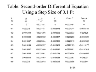
11. 8- 11
0.008373.iserrorThe
1.43296g(1.10)
valueestimatedthesteps,fiveafter0.02,ofsizestepaFor
0.020833.toreducediserrorThe
4205.1])05.1(4)[05.110.1()05.1()10.1(
2.12.01])1(4)[00.105.1()1()05.1(
:)05.1and1(at
twiceequationsr'apply Euleand0.05ofsizestepaUse
value).absolute(in0.04133errorThe
4.1])1(4[1.01)1.1(
getwe,1.0)(ofsizestepaWith
2
2
2
0
=
=−+=
=+=−+=
==
=
=+=
=−=∆
gg
gg
xx
g
xxx

12. 8- 12
Errors with Euler`s Method
• Local error: over one step size.
Global error: cumulative over the range of the solution.
• The error ε using Euler`s method can be approximated using the
second term of the Taylor series expansion as
• If the range is divided into n increments, then the error at the end
of range for x would be nε.
].,[inmaximumtheiswhere
!2
)(
02
2
2
22
0
xx
dx
yd
dx
ydxx −
=ε

13. 8- 13
Example: Analysis of Errors
0088.0)02.0)(1.1)(4(5
022.0)05.0)(1.1)(4(2
044.0)1.0)(1.1(4
:1.1at
errortheonlimitsupperthe0.02.and0.05,0.1,ofsizesstepFor
)(4)8(
!2
)(
byboundediserrortheThus,
8
1at1thatsuch4
2
02.0
2
05.0
2
1.0
2
0
2
0
2
2
2
==
==
==
=
−=
−
=
=
===
ε
ε
ε
ε
x
xxxx
xx
x
dx
yd
xyx
dx
dy

14. 8- 14
Table: Local and Global Errors with a Step Size of 0.1.
x Exact
solution
Numerical
Solution
Local
Error(%)
Global
Error(%)
1 1 1 0 0
1.1 1.4413333 1.4 -2.8677151 -2.8677151
1.2 1.9706667 1.884 -2.300406 -4.3978349
1.3 2.596 2.46 -1.9003595 -5.238829
1.4 3.3253333 3.136 -1.6038492 -5.6936648
1.5 4.1666667 3.92 -1.396 -5-92
1.6 5.128 4.82 -1.1960478 -6.0062402
1.7 6.2173333 5.844 -1.0508256 -6.004718
1.8 7.4426667 7 -0.9315657 -5.947689
1.9 8.812 8.296 -0.8321985 -5.8556514
2 10.333333 9.74 -0.7483871 -5.7419355

15. 8- 15
x Exact
solution
Numerical
Solution
Local
Error(%)
Global
Error(%)
1 1 1 0 0
1.05 1.2101667 1.2 -0.8401047 -0.8401047
1.1 1.4413333 1.4205 -0.7400555 -1.4454209
1.15 1.6945 1.6625 -0.6589948 -1.8884627
1.2 1.9706667 1.927 -0.5920162 -2.2158322
1.25 2.2708333 2.215 -0.5357798 -2.4587156
1.3 2.596 2.5275 -0.4879301 -2.6386749
1.35 2.9471667 2.8655 -0.4467568 -2.771023
1.4 3.3253333 3.23 -0.4109864 -2.8668805
1.45 3.7315 3.622 -0.3796507 -2.9344768
1.5 4.1666667 4.4025 -0.352 -2.98
Table: Local and Global Errors with a Step Size of 0.05.

16. 8- 16
x Exact
solution
Numerica
l Solution
Local
Error(%)
Global
Error(%)
1.55 4.6318333 4.4925 -0.3274441 -3.0081681
1.6 5.128 4.973 -0.3055122 -3.0226209
1.65 5.6561667 5.485 -0.2858237 -3.0261956
1.7 6.2173333 6.0295 -0.2680678 -3.0211237
1.75 6.8125 6.6075 -0.2519878 -3.0091743
1.8 7.4426667 7.22 -0.2373701 -2.9917592
1.85 8.1088333 7.868 -0.2240355 -2.9700121
1.9 8.812 8.5525 -0.2118323 -2.9448479
1.95 9.5531667 9.2745 -0.2006316 -2.9170083
2 10.333333 10.035 -0.1903226 -2.8870968
Table: Local and Global Errors with a Step Size of 0.05
(continued).

17. 8- 17
x Exact solution Numerical Solution Local Error(%) Global Error(%)
1 1 1 0 0
1.02 1.0816107 1.08 -0.1489137 -0.1489137
1.04 1.1664853 1.163232 -0.1408219 -0.2789005
1.06 1.254688 1.24976 -0.1334728 -0.392767
1.08 1.3462827 1.339648 -0.1267688 -0.4928138
1.1 1.4413333 1.43296 -0.120629 -0.5809436
1.2 1.9706667 1.95312 -0.0963464 -0.8903924
1.3 2.596 2.56848 -0.0793015 -1.0600924
1.4 3.3253333 3.28704 -0.0667201 -1.1515638
1.5 4.1666667 4.1168 -0.057088 -1.1968
1.6 5.128 5.06876 -0.049506 -1.2137285
1.7 6.2173333 6.14192 -0.0434055 -1.212953
1.8 7.4426667 7.35328 -0.0384092 -1.2010032
1.9 8.812 8.70784 -0.0342563 -1.1820245
2 10.333333 10.2136 -0.0307613 -1.1587097
Table: Local and Global Errors with a Step Size of 0.02.

18. 8- 18
Modified Euler’s Method
• Use an average slope, rather than the slope at the start
of the interval :
a. Evaluate the slope at the start of the interval
b. Estimate the value of the dependent variable y at the
end of the interval using the Euler’s metod.
c. Evaluate the slope at the end of the interval.
d. Find the average slope using the slopes in a and c.
e. Compute a revised value of the dependent variable y
at the end of the interval using the average slope of
step d with Euler’s method.

19. 8- 19
Example : Modified Euler’s Method
1at1thatsuch === xyyx
dx
dy
10768.1)07684.1(1.01)0.11.1()0.1()1.1(1e.
07684.1)15369.11(
2
1
1d.
15369.11.11.1c.1
1.1)1(1.01)0.11.1()0.1()1.1(1b.
111a.1
:1.0foriterationfirsttheofstepsfiveThe
1.1
1
1
=+=−+=
=+=
==
=+=−+=
==
=∆
a
a
dx
dy
gg
dx
dy
dx
dy
dx
dy
gg
dx
dy
x

20. 8- 20
23193.1)1.12.1()1.1()2.1(2e.
24251.1)(
2
1
2d.
32732.122345.12.1c.2
22345.1)15771.1(1.010768.1)1.12.1()1.1()2.1(2b.
15771.110768.11.1a.2
:intervalsecondfor thestepsThe
2.11.1
2.1
1.1
1.1
=−+=
=+=
==
=+=−+=
===
a
a
dx
dy
gg
dy
dx
dy
dx
dy
dx
dx
dy
dx
dy
gg
yx
dx
dy

21. 8- 21
Second-order Runge-Kutta Methods
• The modified Euler’s method is a case of the second-
order Runge-Kutta methods. It can be expressed as
xhxxx
xxgyxgy
hyxhfyhxfyxfyy
ii
iiii
iiiiiiii
∆=∆+=
∆+==
++++=
+
+
+
,
),(),(where
))],(,(),([5.0
1
1
1

22. 8- 22
• The computations according to Euler’s method:
1. Evaluate the slope at the start of an interval, that is,
at (xi,yi) .
2. Evaluate the slope at the end of the interval (xi+1,yi+1) :
3. Evaluate yi+1 using the average slope S1 of and S2 :
),(1 ii yxfS =
),( 12 hSyhxfS ii ++=
hSSyy ii )(5.0 211 ++=+

23. 8- 23
Third-order Runge-Kutta Methods
• The following is an example of the third-order Runge-
Kutta methods :
hyxhfyhxhfyxhfyhxf
yxhfyhxfyxfyy
iiiiiiii
iiiiiiii
)))],(5.0,5.0(2),(,(
)),(5.0,5.0(4),([
6
1
1
+++−+
+++++=+

24. 8- 24
• The computational steps for the third-order method:
1. Evaluate the slope at (xi,yi).
2. Evaluate a second slope S2 estimate at the mid-point
in of the step as
3. Evaluate a third slope S3 as
4. Estimate the quantity of interest yi+1 as
)5.0,5.0( 12 hSyhxfS ii ++=
)2,( 213 hShSyhxfS ii +−+=
hSSSyy ii ]4[
6
1
3211 +++=+
),(1 ii yxfS =

25. 8- 25
Fourth-order Runge-Kutta Methods
1. Compute the slope S1 at (xi,yi).
2. Estimate y at the mid-point of the interval.
3. Estimate the slope S2 at mid-interval.
4. Revise the estimate of y at mid-interval
.atthatsuch),( 00 hxxxyyyxf
dx
dy
=∆===
),(1 ii yxfS =
),(
2
2/1 iiii yxf
h
yy +=+
)5.0,5.0( 12 hSyhxfS ii ++=
22/1
2
S
h
yy ii +=+

26. 8- 26
5. Compute a revised estimate of the slope S3 at mid-
interval.
6. Estimate y at the end of the interval.
7. Estimate the slope S4 at the end of the interval
8. Estimate yi+1 again.
)5.0,5.0( 23 hSyhxfS ii ++=
31 hSyy ii +=+
),( 34 hSyhxfS ii ++=
)22(
6
43211 SSSS
h
yy ii ++++=+

27. 8- 27
Predictor-Corrector Methods
• Unless the step sizes are small, Euler’s method
and Runge-Kutta may not yield precise
solutions.
• The Predictor-Corrector Methods iterate
several times over the same interval until the
solution converges to within an acceptable
tolerance.
• Two parts: predictor part and corrector part.

28. 8- 28
Euler-trapezoidal Method
• Euler’s method is the predictor algorithm.
• The trapezoidal rule is the corrector equation.
• Eluer formula (predictor):
• Trapezoidal rule (corrector):
The corrector equation can be applied as many times as
necessary to get convergence.
,*
,*,1
i
iji
dx
dy
hyy +=+
][
2 1,1,*
,*,1
−+
+ ++=
jii
iji
dx
dy
dx
dyh
yy

29. 8- 29
Example 8-6: Euler-trapezoidal Mehtod
1at1thatsuch:Problem === xyyx
dx
dy
1.1)1(1.01
1.0
111
is1.1atforestimate)(predictorinitialThe
0,1
0,0
,*00,1
0,0
=+=






+=
==
=
y
dx
dy
yy
dx
dy
xy
15369.11.11.1
:estimatetheimprovetousedisequationcorrectorThe
0,1
==
dx
dy

30. 8- 30
[ ]
[ ]
[ ] 10789.115782.11
2
1.0
1
2
15782.110789.11.1
10789.115771.11
2
1.0
1
2
15771.110768.11.1
10768.115369.11
2
1.0
1
2
2,10,0
,*03,1
2,1
1,10,0
,*02,1
1,1
0,10,0
,*01,1
=++=





++=
==
=++=





++=
==
=++=





++=
dx
dy
dx
dyh
yy
dx
dy
dx
dy
dx
dyh
yy
dx
dy
dx
dy
dx
dyh
yy
.haveweAnd
.1.1at1.10789toconverges,Since
3,1,*1
2,13,1
yy
xyyy
=
==

31. 8- 31
22367.1)15782.1(1.010789.1
:equationpredictorthe,2.1atofestimateFor the
,*1,*10,2 =+=+=
=
dx
dy
hyy
xy
[ ]
33203.123215.12.1
23215.132744.115782.1
2
1.0
10789.1
2
32744.122367.12.1
:equationcorrectorThe
2,2
1,2,*1
,*11,2
1,2
==
=++=






++=
==
dx
dy
dx
dy
dx
dyh
yy
dx
dy

32. 8- 32
[ ]
[ ]
1.23239.is2.1atofestimateThe
.iterationsthreeinconvergesalgorithmcorrectortheAgain,
23239.133215.115782.1
2
1.0
10789.1
2
33215.123238.12.1
23238.133203.115782.1
2
1.0
10789.1
2
3,2,*1
,*13,2
3,2
2,2,*1
,*12,2
=
=++=






++=
==
=++=






++=
xy
dx
dy
dx
dyh
yy
dx
dy
dx
dy
dx
dyh
yy

33. 8- 33
Milne-Simpson Method
• Milne’s equation is the predictor euqation.
• The Simpson’s rule is the corrector formula.
• Milne’s equation (predictor):
For the two initial sampling points, a one-step
method such as Euler’s equation can be used.
• Simpsos’s rule (corrector):
]22[
3
4
,*2,*1,*
,*30,1
−−
−+ +−+=
iii
ii
dx
dy
dx
dy
dx
dyh
yy
]4[
3 ,*1,*,1
,*1,1
−+
−+ +++=
iiji
iji
dx
dy
dx
dy
dx
dyh
yy

34. 8- 34
Example 8-7: Milne-Simpson Mehtod
.4.1and3.1atestimatewant toWe
1at1thatsuch:Problem
==
===
xxy
xyyx
dx
dy
1 1 1
1.1 1.10789 1.15782
1.2 1.23239 1.33215
Assume that we have the following values,
obtained from the Euler-trapezoidal method
in Example 8-6.
x y dx
dy

35. 8- 35
51917.136560.13.1
36560.1)33215.1(1.023239.1
:usedbecanmethodsEuler'
,3.1atforestimate)(predictorinitialthecomputeTo
0,3
,*2
,*20,3
==
=+=+=
=
dx
dy
dx
dy
hyy
xy
[ ]
37474.1
15782.1)33215.1(451917.1
3
1.0
10789.1
4
3
1.0
:formularcorrectorThe
,*1,*20,3
,*11,3
=
+++=






+++=
dx
dy
dx
dy
dx
dy
yy

36. 8- 36
[ ]
[ ]
37492.1
15782.1)33215.1(452434.1
3
1.0
10789.1
52434.137491.13.1
37491.1
15782.1)33215.1(452424.1
3
1.0
10789.1
52424.137474.13.1
3,3
2,3
2,3
1,3
=
+++=
==
=
+++=
==
y
dx
dy
y
dx
dy
The computations for x=1.3 are complete.

37. 8- 37
The Milne predictor equation for estimating y at x=1.4:
( ) ( ) ( )[ ]
53762.1
15782.1233215.152434.12
3
1.04
1
22
3
4
,*1,*2,*3
,*00,4
=
+−+=






+−+=
dx
dy
dx
dy
dx
dyh
yy
73610.153762.14.1
1,4
==
dx
dy
The corrector formular:

38. 8- 38
( )[ ]
( )[ ]
complete.isitThen
53791.133215.152434.1473617.1
3
1.0
23239.1
73617.153791.14.1
53791.1
33215.152434.1473601.1
3
1.0
23239.1
4
3
2,4
2,4
,*2,*30,4
,*21,4
=+++=
==
=
+++=






+++=
y
dx
dy
dx
dy
dx
dy
dx
dyh
yy

39. 8- 39
Least-Squares Method
• The procedure for deriving the least-squares
function:
1. Assume the solution is an nth-order polynomial:
2. Use the boundary condition of the ordinary
differential equation to evaluate one of (bo,b1,b2,
…,bn).
3. Define the objective function:
n
nx xbxbbby ++++= 2
210ˆ
dxeF
x∫= 2
dx
dy
dx
yd
e −=
ˆ
where

40. 8- 40
4. Find the minimum of F with respect to the unknowns
(b1,b2, b3,…,bn) , that is
5. The integrals in Step 4 are called the normal
equations; the solution of the normal equations yields
value of the unknowns (b1,b2, b3,…,bn).
∫ =
∂
∂
=
∂
∂
xall
ii
dx
b
e
e
b
F
02

41. 8- 41
Example 8-8: Least-squares Method
2/2
:solutionAnalytical
1.x0intervalfor theitSolve
0at1thatsuch:Problem
x
ey
xyxy
dx
dy
=
≤≤
===
1
1
0
10
10
ˆ
1ˆ
ismodellineartheThus.1yields
)0(1ˆ
conditionboundarytheUsing
ˆ
b
dx
yd
xby
b
bby
xbby
=
+=
=
+==
+=
• First, assume a linear model is used:

42. 8- 42
0)
543
2
2
(
0)1)](1([22
1
)1(
:functionerrorThe
0
5
1
43
1
2
1
0 0
2
11
1
2
1
111
=++−−
=−+−=
−=
+−=−=
∫ ∫
x
x x
xbxxbx
xb
dxxxbxbdx
db
de
e
x
db
de
xbxbxybe
xy
x
x
32
15
32
15
1
1ˆ
Thus,.bgetwe,1withintegralabove
thesolve,10rangetheininterestedareweSince
+=
==
≤≤

43. 8- 43
x True y Value Numerical y Value Error (%)
0 1. 1. -
0.2 1.0202 1.0938 7.2
0.4 1.0833 1.1875 9.6
0.6 1.1972 1.2812 7.0
0.8 1.3771 1.3750 0.0
1.0 1.6487 1.46688 -10.9
Table: A linear model for the least-squares method
2/2
x
ey = xy 32
15
1ˆ +=

44. 8- 44
• Next, to improve the accuracy of estimates, a
quadratic model is used:
xxxbxb
xbxbxxbbxyxbbe
xbb
dx
yd
b
bbby
xbxbby
−−+−=
++−+=−+=
+=
=
++==
++=
)2()1(
)1(22
isfunctionerrorThe
2
ˆ
.1yields
)0()0(1ˆ
conditionboundarytheUsing
ˆ
3
2
2
1
2
212121
21
0
2
210
2
210

45. 8- 45
( ) ( )[ ]( )
4
1
12
5
15
8
:limituppertheas1Using
0
46524
3
3
2
0121
1
21
0
46
2
5
1
24
22
2
3
1
1
0
23
2
2
1
2
1
=+
=
=





+++−−+−
=−−−+−
−=
∂
∂
∫
bb
x
xxbxbxxb
xb
xb
xb
dxxxxxbxb
x
b
e
x
x

46. 8- 46
( ) ( )[ ]( )
2
21
21
0
57
2
5
1
25
2
4
2
4
12
1
0
33
2
2
1
3
2
78776.014669.01ˆ
.78776.0and14669.0getWe
15
7
105
71
20
9
:limituppertheas1Using
0
5753
2
5
4
3
4
4
2
02212
2
xxy
bb
bb
x
xxbxbxxbxbxb
xb
dxxxxxxbxb
xx
b
e
x
x
+−=
=−=
=+
=
=





+++−−+−
=−−−+−
−=
∂
∂
∫

47. 8- 47
x True y Value Numerical y Value Error (%)
0 1. 1. -
0.2 1.0202 1.0022 -1.8
0.4 1.0833 1.0674 0.0
0.6 1.1972 1.1956 0.0
0.8 1.3771 1.38668 0.0
1.0 1.6487 1.6411 0.0
Table: A quadratic model for the least-squares method
2/2
x
ey = 2
78776.014669.01ˆ xxy +−=

48. 8- 48
Galerkin Method
• Example: Galerkin Method
The same problem as Example 8-8.
Use the quadratic approximating equation.
i
i
i
x
i
b
e
w
w
niedxw
∂
∂
=
==∫
method,squaresleastFor the
factor.nga weightiiswhere
...2,10
.andLet 2
21 xwxw ==

49. 8- 49
2
21
21
1
0
23
2
2
1
1
0
3
2
2
1
85526.026316.01ˆ
:resultfinalThe
4
1
3
1
15
2
3
1
15
7
12
1
:equationsnormalfollowingget theWe
0])2()1([
0])2()1([
xxy
bb
bb
dxxxxxbxb
xdxxxxbxb
+−=
=+
=+
=−−+−
=−−+−
∫
∫

50. 8- 50
Table: Example for the Galerkin method
x True y value Numerical y value Error
(%)
0 1. 1. --
0.2 1.0202 0.9816 0.0
0.4 1.0833 1.0316 0.0
0.6 1.1972 1.1500 0.0
0.8 1.3771 1.3368 0.0
1.0 1.6487 1.5921 0.0
2/2
x
ey = 2
85526.026316.01ˆ xxy +−=

51. 8- 51
Higher-Order Differential Equations
• Second order differential equation:
Transform it into a system of first-order differential
equations.
dx
dy
dx
dy
yyy
y
dx
dy
yyxf
dx
dy
===
=
=
1
21
2
1
21
2
andwhere
),,(






=
dx
dy
yxf
dx
yd
,,2
2

52. 8- 52
• In general, any system of n equations of the following
type can be solved using any of the previously
discussed methods:
),...,,(
),...,,(
),...,,(
),...,,(
21
213
3
212
2
211
1
nn
n
n
n
n
yyyxf
dx
dy
yyyxf
dx
dy
yyyxf
dx
dy
yyyxf
dx
dy
=
=
=
=


53. 8- 53
Example: Second-order Differential Equation
EI
XX
EI
M
dX
Yd 2
2
2
10
:Problem
−
==
Z
dX
dY
EI
XX
EI
M
dX
dZ
=
−
==
10
:intomedtransforbecanIt
2
hZYXfYY
hZYXfZZ
ZYXEI
iiiii
iiiii
),,(
),,(
:equationsfollowingthesolvetomethodsEuler'Use
02314.0and0,0at3600Assume
11
21
+=
+=
−====
+
+

54. 8- 54
Table: Second-order Differential Equation
Using a Step Size of 0.1 Ft
X
(ft)
Y
(ft)
Exact Z Exact Y
(ft)
0 0 -0.0231481 0 -0.0231481 0
0.1 0.000275 -0.0231481 -0.0023148 -0.0231344 -0.0023144
0.2 0.0005444 -0.0231206 -0.0046296 -0.0230933 -0.004626
0.3 0.0008083 -0.0230662 -0.0069417 -0.0230256 -0.0069321
0.4 0.0010667 -0.0229854 -0.0092483 -0.0229319 -0.0092302
0.5 0.0013194 -0.0228787 -0.0115469 -0.0228125 -0.0115177
0.6 0.0015667 -0.0227468 -0.0138347 -0.0226681 -0.0137919
0.7 0.0018083 -0.0225901 -0.0161094 -0.0224994 -0.0160505
0.8 0.0020444 -0.0224093 -0.0183684 -0.0223067 -0.018291
0.9 0.002275 -0.0222048 -0.0206093 -0.0220906 -0.020511
dX
dZ
dX
dY
Z =

55. 8- 55
Table: Second-order Differential Equation
Using a Step Size of 0.1 Ft (continued)
dX
dZ
dX
dY
Z =
X
(ft)
Y
(ft)
Exact Z Exact Y
(ft)
1 0.0025 -0.0219773 -0.0228298 -0.0218519 -0.0227083
2 0.0044444 -0.0185565 -0.0434305 -0.0183333 -0.04296663
3 0.0058333 -0.0134412 -0.0298019 -0.0131481 -0.0588194
4 0.0066667 -0.007187 -0.0704998 -0.0068519 -0.0688889
5 0.0069444 -0.0003495 -0.0746352 0.00000000 -0.071228
6 0.0066667 0.0065157 -0.0718747 0.0068519 -0.0688889
7 0.0058333 0.0128532 -0.06244066 0.0131481 -0.0588194
8 0.0044444 0.0181074 -0.0471107 0.0183333 -0.042963
9 0.0025 0.0217227 -0.0272183 0.0278519 -0.0227083
10 0.000000 0.0231435 -0.00466523 0.0231481 0.000000