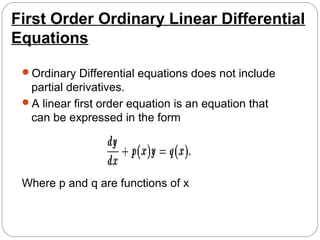
This document contains a summary of a student group project on first order ordinary differential equations (ODEs). It defines key terms related to ODEs such as order, degree, general solutions, and singular solutions. It also categorizes common types of first order ODEs including separable, homogeneous, exact, and linear equations. Solution methods are described for each type. Additional topics covered include Bernoulli equations, orthogonal trajectories, and applications of ODEs in areas like radioactivity, electrical circuits, economics, and physics. The document is authored by six chemical engineering students at G.H. Patel College of Engineering and Technology.

1. G.H.PATEL COLLEGE OF ENGINEERING AND TECHNOLOGY
Chemical Department
Topic Name: First Order ODE with Application
Subject: Advanced Engineering Mathematics(2130002)
Name:
Shivam Patel (150110105031)
Vatsal Patel (150110105032)
Vyom Patodiya (150110105033)
Krishna Peshivadiya (150110105034)
Hardik Pipaliya (150110105035)
Bhavin Poshiya (150110105036).
Faculty Name: Prof. Mukesh T. Joshi

2. Content:
Introduction
Some useful Terms
Type of First Order ODEs
Bernoulli Equation
Orthogonal Trajectory

3. First Order Ordinary Linear Differential
Equations
Ordinary Differential equations does not include
partial derivatives.
A linear first order equation is an equation that
can be expressed in the form
Where p and q are functions of x

4. Some useful Terms:
First order differential equation with y as the
dependent variable and x as the independent
variable would be:
Second order differential equation will have the
form:
( )
dy
f x,y
dx
=
),,(2
2
dx
dy
yxf
dx
yd
=

5. The order of a differential equation is the order of the
highest derivative occurring in the equation.
The degree of a differential equation is the power of
the highest ordered derivative occurring in the
equation, provided all derivatives are made free from
radicals and fractions.
• Uniqueness: Does a differential equation have more than
one solution? If yes, how can we find a solution which
satisfies particular conditions?

6. If no initial conditions are given, we call the
description of all solutions to the differential equation
the general solution. This type of solution will contain
arbitrary constants whose number is equal to the
order of differential equation.
A solution obtained from the general solution by
giving particular values to arbitrary constants is
known as a particular solution.
A solution which cannot be obtained from general
solution is called a singular solution.

7. Types Of First 0rder ODE:
1. Variable Separable
2. Homogeneous Differential Equation
3. Exact Differential Equation
4. Linear Differential Equation

8. The first-order differential equation
( ),
dy
f x y
dx
=
is called separable provided that f(x,y) can be written
as the product of a function of x and a function of y.
(1)
1. Variable Separation:-

9. Suppose we can write the above equation as
)()( yhxg
dx
dy
=
We then say we have “ separated ” the variables. By
taking h(y) to the LHS, the equation becomes

10. 1
( )
( )
dy g x dx
h y
=
Integrating, we get the solution as
1
( )
( )
dy g x dx c
h y
= +∫ ∫
where c is an arbitrary constant.

11. Example 1. Consider the D.E. y
dx
dy
=
Sol. Separating the variables, we get
dxdy
y
=
1
Integrating we get the solution as
kxy +=||ln
or ccey x
,= an arbitrary constant.

12. 2. Homogeneous Diff. equations
Definition : A function f(x, y) is said to be
homogeneous of degree n in x, y if
),(),( yxfttytxf n
= for all t, x, y
Examples
22
2),( yxyxyxf −−=
is homogeneous of degree
)sin(),(
x
xy
x
y
yxf
−
+=
is homogeneous of degree
2.
0.

13. A first order D.E. 0),(),( =+ dyyxNdxyxM
is called homogeneous if ),(,),( yxNyxM
are homogeneous functions of x and y of the same
degree.
This D.E. can be written in the form
),( yxf
dx
dy
=
The substitution y = vx converts the given equation into
“variables separable” form and hence can be solved.
(Note that v is also a new variable)

14. Working Rule to solve homogeneous ODE:
1. Put the given equation in the form
.Let.3 zxy =
)1(0),(),( =+ dyyxNdxyxM
2. Check M and N are Homogeneous function of the
same degree.

15. 5. Put this value of dy/dx into (1) and solve the equation
for z by separating the variables.
6. Replace z by y/x and simplify.
dx
dz
xz
dx
dy
+=
4. Differentiate y = z x to get

16. Example:- Solve the Homogeneous ODE
)sin(
x
xy
x
y
y
−
+=′
Let y = z x. Hence we get
zz
dx
dz
xz sin+=+ or z
dx
dz
x sin=
Separating the variables, we get
x
dx
dz
z
=
sin
1
Integrating we get
where
cosec z – cot z = c x
and c an arbitrary constant.
y
z
x
=

17. 3. EXACT DIFFERENTIAL EQUATIONS
A first order D.E. 0),(),( =+ dyyxNdxyxM
is called an exact D.E. if
M N
y x
∂ ∂
=
∂ ∂
The solution given by:
∫ ∫ =+ cNdyMdx
(Terms free from ‘x’)

18. Solution is:
cyxy
cdy
y
ydx
=+
=+∫ ∫
ln2
2
∫ ∫ =+ cNdyMdx

19. Example 1 The D.E. 0xdx y dy+ =
Sol.:- It is exact as it is d (x2
+ y2
) = 0
Hence the solution is: x2
+ y2
= c
Example 2 The D.E. 2
1
sin( ) sin( ) 0
x x x
dx dy
y y y y
− + =
Sol:- It is exact (cos( )) 0
x
d
y
=
Hence the solution is: cos( )
x
c
y
=

20. Integrating Factors
Definition: If on multiplying by I.F.(x, y) or µ, the D.E.
0M dx N dy+ =
becomes an exact D.E. , we say that I.F.(x, y) or µ is an
Integrating Factor of the above D.E.
2 2
1 1 1
, ,
xy x y
are all integrating factors of
the non-exact D.E. 0y dx xdy− =

21. ( )
M N
y x
g x
N
∂ ∂
−
∂ ∂
=
( )g x dx
eµ ∫=
is an integrating factor of the given DE
0M dx N dy+ =
Rule 1: I.F is a function of ‘x’ alone.

22. Rule 2: I.F is a function of ‘y’ alone.
If , a function of y alone,
then
( )h y dy
eµ ∫=
is an integrating factor of the given DE.
x
N
y
M
∂
∂
−
∂
∂
M
( )yh=

23. is an integrating factor of the given DE
0M dx N dy+ =
Rule 3: Given DE is homogeneous.
µ=
+ NyMx
1

24. Rule 4: Equation is of the form of
( ) ( ) 021 =+ xdyxyfydxxyf
Then,
NyMx −
=
1
µ

25. Example 1 Find an I.F. for the following DE
and hence solve it.
2
( 3 ) 2 0x y dx xydy+ + =
Sol.:-Here
6 2
M N
y y
y x
∂ ∂
= ≠ =
∂ ∂
2
( 3 ); 2M x y N xy= + =
Hence the given DE is not exact.

26. M N
y x
N
∂ ∂
−
∂ ∂
=Now 6 2
2
y y
xy
−
=
2
( ),g x
x
=
a function of x alone. Hence
( )g x dx
eµ ∫= =
2
2
dx
x
e x
∫
=
is an integrating factor of the given DE
Multiplying by x2
, the given DE becomes

27. 3 2 2 3
( 3 ) 2 0x x y dx x ydy+ + =
which is of the form 0M dx N dy+ =
Note that now 3 2 2 3
( 3 ); 2M x x y N x y= + =
Integrating, we easily see that the solution is
4
3 2
,
4
x
x y c+ = c an arbitrary constant.

28. 4. Linear Diff. Equations
A linear first order equation is an equation that can be
expressed in the form
1 0( ) ( ) ( ), (1)
dy
a x a x y b x
dx
+ =
where a1(x), a0(x), and b(x) depend only on the
independent variable x, not on y.

29. We assume that the function a1(x), a0(x), and b(x) are
continuous on an interval and that a1(x) ≠ 0on that
interval. Then, on dividing by a1(x), we can rewrite
equation (1) in the standard form
( ) ( ) (2)
dy
P x y Q x
dx
+ =
where P(x), Q(x) are continuous functions on the interval.

30. Rules to solve a Linear D.E.:-
1. Write the equation in the standard form
( ) ( )
dy
P x y Q x
dx
+ =
2. Calculate the IF µ(x) by the formula
( )( ) exp ( )x P x dxµ = ∫
3. Multiply the equation by µ(x).
4. Integrate the last equation.

31. Example 1. Solve
( ) 1cossincos =++





xxxy
dx
dy
xx
Solution :- Dividing by x cos x, throughout, we get
x
x
y
x
x
dx
dy sec1
tan =





++

32. 1
tan( )
( )
x dxP x dx x
x e eµ
 
 ÷
 
+∫∫= =
log sec log loglog sec
( ) sece e ex x xx
x e e e x xµ +
= = =
( )
sec
sec sec
d x
dx x
y x x x x=
2
sec sec tany x xdx C x C= + = +∫
Multiply by secx x so
Integrate both side we get

33. Bernoulli Equation
In mathematics, an ordinary differential equation of the
form:
y'+P(x)y=Q(x)y^{n}
is called a Bernoulli differential equation where { n} is
any real number and n≠ 0 or n ≠1. It is named
after Jacob Bernoulli who discussed it in 1695.
Bernoulli equations are special because they are
nonlinear differential equations with known exact
solutions.

34. before.toldweassolutionitsandequationlinearisthis
)()1()()1(
)()(
)1(
1
)1(thenPutb)
)()(
1
yoverEquationBernoulliDividea)
EquationBernoullisolveTo
)1(
)1(
n
xQnzxpn
dx
dz
xQxp
dx
dz
n
dx
dy
yn
dx
dz
yz
xQyxP
dx
dy
y
n
n
n
−=−+
=+
−
∴
−==
=+
−
−
note :-
if n = 0 the Bernoulli
Equation will be
linear equation.
if n = 1 Bernoulli
Equation will be
separable equation

35. the general solution will be
2
22
1
2
lnexpln2expexpexp
linearisequationthissin62
22
.sin3
solution
sin3)
x
xxdxpdx
x
x
z
dx
dz
dx
dy
y
dx
dz
enand thyput z
yx
x
y
–
dx
dy
x
x
y
–
dx
dy
yEx
x
=∴
====
=+
==
=
=
∫∫
−
µ
µ
cxxxxyx
cxdxxyx
+++−=
+∫=
)cossincos(6
sin6
22
22

36. Orthogonal Trajectories
Orthogonal trajectories are a
family of curves in the plane
that intersect a given family of
curves at right angles.
Suppose we are given the
family of circles centered
about the origin:
x2
+ y2
= c
The orthogonal trajectories of
this family are the family of
curves/lines such that
intersect the circle at right
angles.

37. Example
Find the orthogonal trajectories of the curve x2
+
y2
= c2
Solution:-Differentiating w.r.t. variable x, we get
Writing it in explicit form, we get

38. The derived equation is a linear equation.
If we use the method of solving linear equations, then we derive
the following results for I.F. :
Thus, we get the general solution as
y = mx

39. General Applications of ODE
ODEs are used in various fields such as:
Radioactivity and carbon dating
Equations of series RL circuits
Economics
Bernoulli Equation
Population Dynamics
Newton’s Law of Cooling

40. •Cooling/Warming law
We have seen in Newton’sempirical law of cooling of
an object in given by the linear first-order differential
equation
)mTα(T
dt
dT
−=
This is a separable differential equation. We have
αdt
)T(T
dT
m
=
−
or ln|T-Tm
|
=αt+c1
or T(t) = Tm
+c2
eαt

41. In Series Circuits
i(t), is the solution of the differential equation.
)(tERi
dt
di
=+Ι
dt
dq
i =
)t(Eq
C
1
dt
dq
R =+
Si
nce
It can be
written as