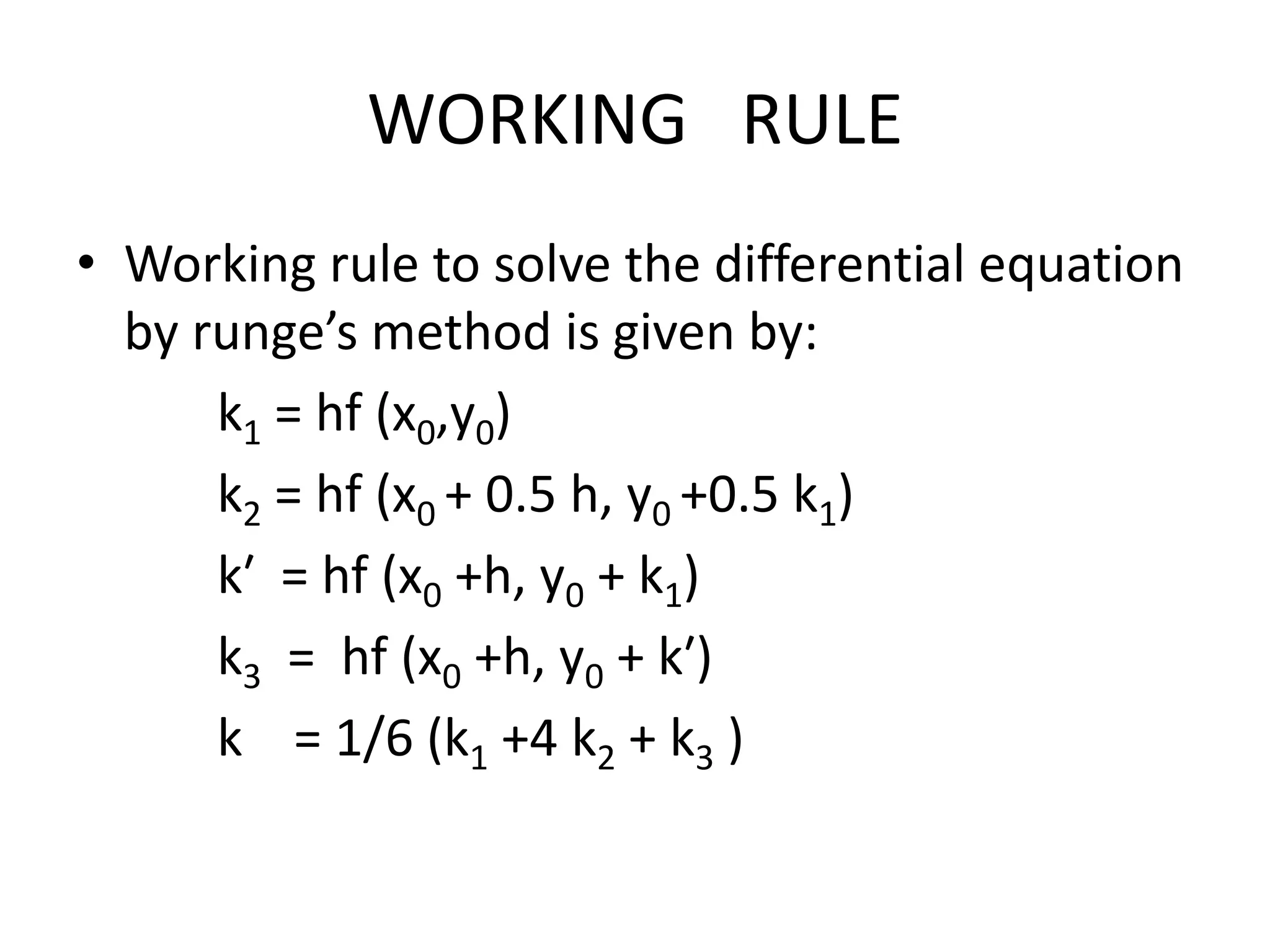
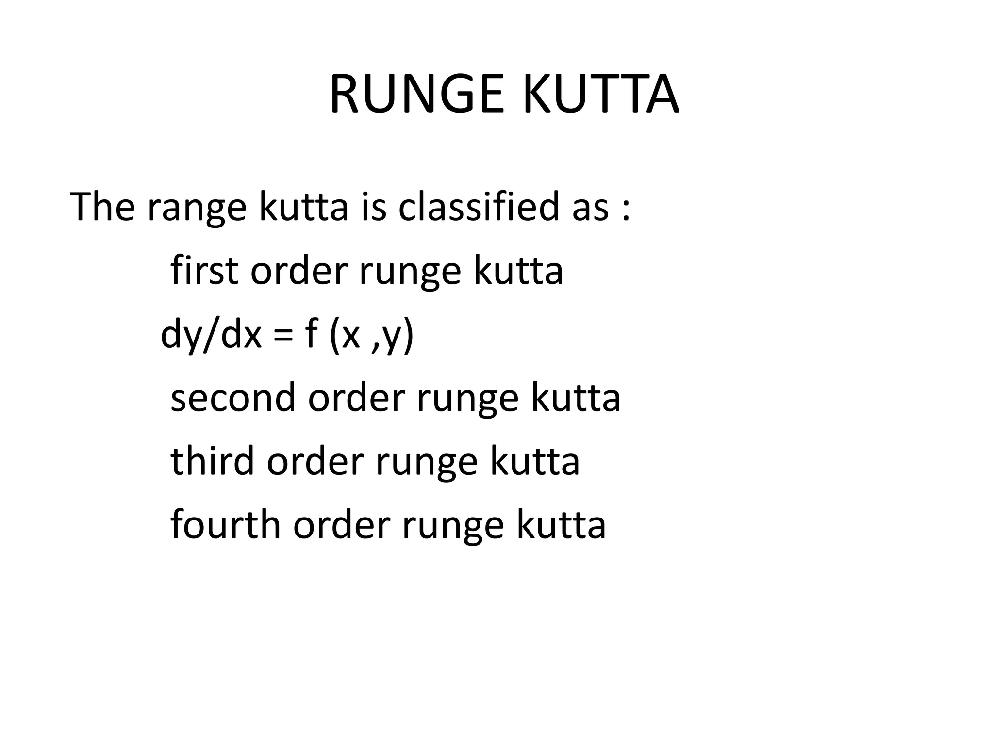
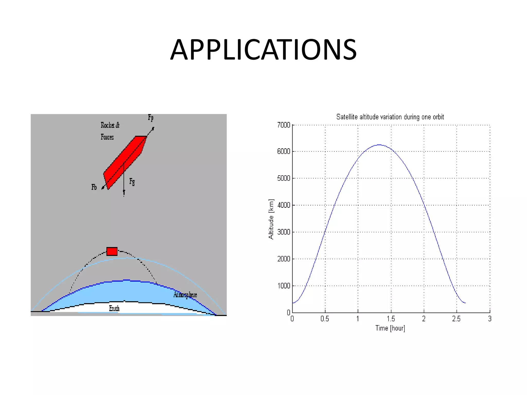
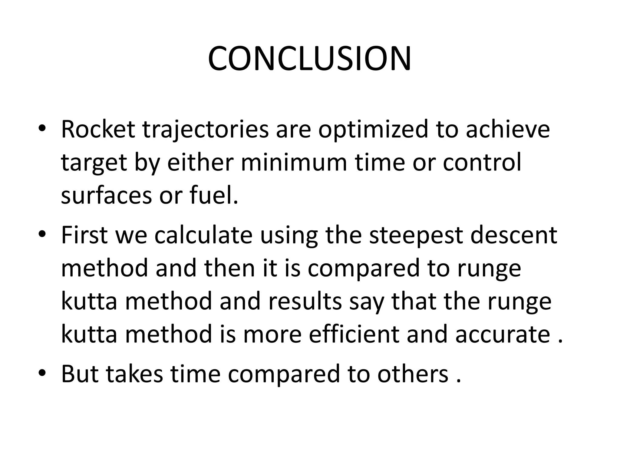
The document discusses numerical methods for solving first-order ordinary differential equations, particularly focusing on the Runge-Kutta methods introduced by mathematicians Runge and Kutta. These methods are noted for their accuracy and efficiency in calculating solutions for applications such as rocket trajectories. The conclusion emphasizes the superiority of the Runge-Kutta method in optimizing rocket paths, despite a longer computation time compared to other methods.

1. NUMERICAL SOLUTION OF
ORDINARY DIFFERENTIAL EQUATION
BY Dixi patel

2. INTRODUCTION
• A number of numerical methods are available
for the solution of first order differential
equation of form:
• dy/ dx = f(x ,y)
• These methods yield solution either as power
series or in x form which the values of y can be
found by direct substitution, or a set of values
of x and y.

3. NUMERICAL METHODS
• The numerical methods for ODE include:
Picard
Taylor series
Euler series
Runge-kutta methods
Milne
Adams-Bashforth

4. RUNGE-KUTTA METHOD
• For the first time, the methods were
presented by Runge and Kutta two German
mathematicians.
• These methods were very accurate and
efficient and instead direct calculation of
higher derivatives only function used for
different values.

5. WORKING RULE
• Working rule to solve the differential equation
by runge’s method is given by:
k1 = hf (x0,y0)
k2 = hf (x0 + 0.5 h, y0 +0.5 k1)
k′ = hf (x0 +h, y0 + k1)
k3 = hf (x0 +h, y0 + k′)
k = 1/6 (k1 +4 k2 + k3 )

6. BASIC GRAPH

7. RUNGE KUTTA
The range kutta is classified as :
first order runge kutta
dy/dx = f (x ,y)
second order runge kutta
third order runge kutta
fourth order runge kutta

8. APPLICATIONS

9. APPLICATIONS
• If a model rocket is prepared this method can
be used for successive iterations of the
differential equations for lift off the rocket.
• Runge kutta method is used to know the
ballistic missile trajectory of a rocket.
• In the study of self propelled missiles.

10. CONCLUSION
• Rocket trajectories are optimized to achieve
target by either minimum time or control
surfaces or fuel.
• First we calculate using the steepest descent
method and then it is compared to runge
kutta method and results say that the runge
kutta method is more efficient and accurate .
• But takes time compared to others .

11. THANK YOU