Downloaded 128 times


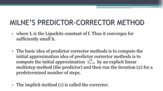

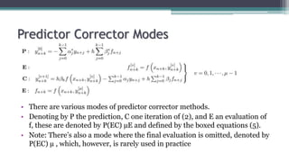
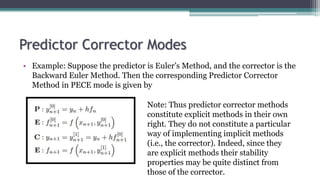
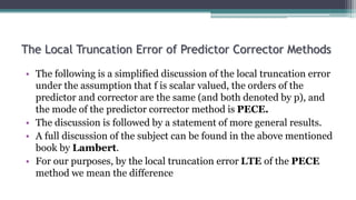
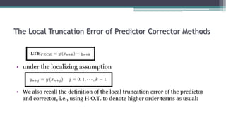
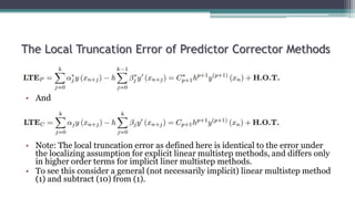
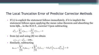

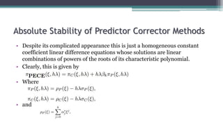

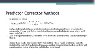
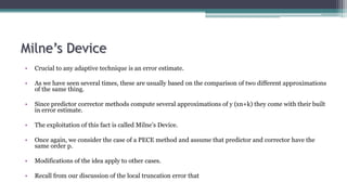
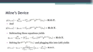


This document discusses Milne's predictor-corrector method for solving ordinary differential equations. Predictor-corrector methods use an explicit method (the predictor) to get an initial approximation, followed by iterations of an implicit method (the corrector) to refine the solution. Milne's method provides a built-in error estimate by comparing the predictor and corrector approximations, allowing for adaptive step size control. The document outlines the local truncation error and absolute stability properties of predictor-corrector methods.