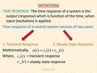
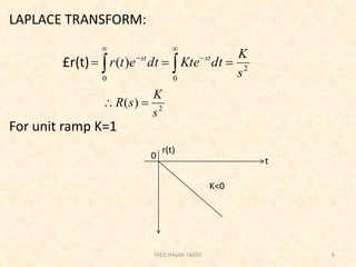
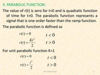
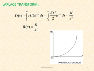
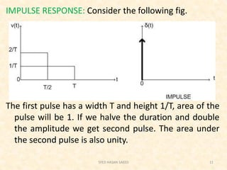
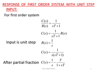
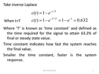
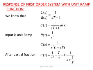
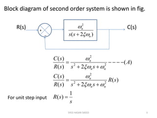
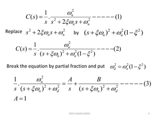
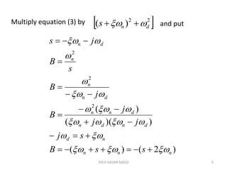
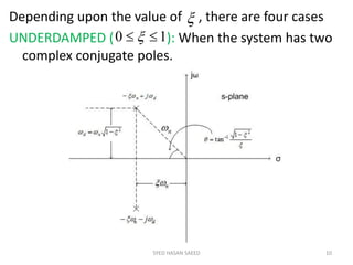
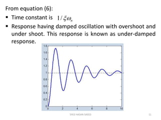
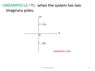
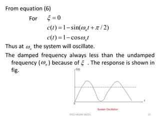
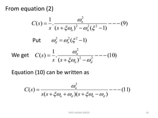
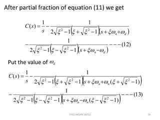
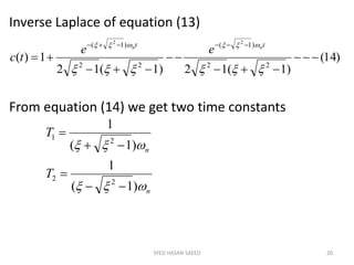
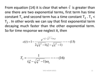
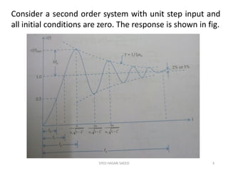
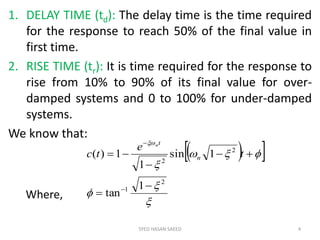
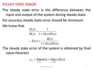
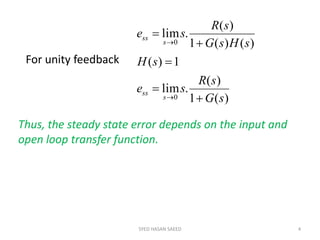
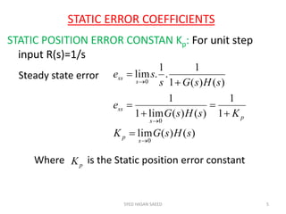
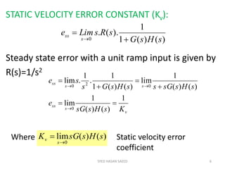
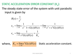
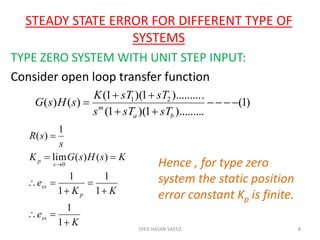
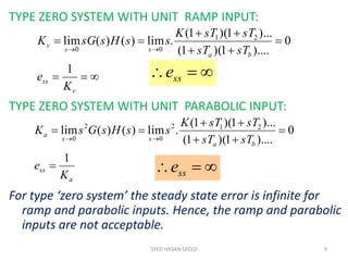
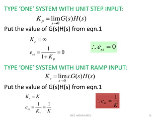
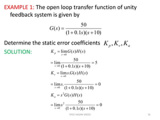
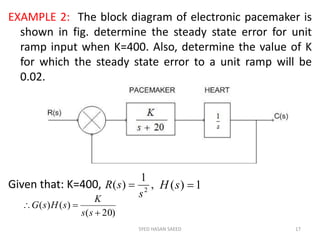
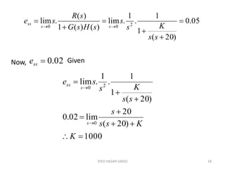
TIME DOMAIN ANALYSIS

TIME DOMAIN ANALYSIS
Email: hasansaeedcontrol@gmail.com
URL: http://shasansaeed.yolasite.com/
1SYED HASAN SAEED

BOOKS
1. AUTOMATIC CONTROL SYSTEM KUO & GOLNARAGHI
2. CONTROL SYSTEM ANAND KUMAR
3. AUTOMATIC CONTROL SYSTEM S.HASAN SAEED
SYED HASAN SAEED 2

DEFINITIONS
TIME RESPONSE: The time response of a system is the
output (response) which is function of the time, when
input (excitation) is applied.
Time response of a control system consists of two parts
1. Transient Response 2. Steady State Response
Mathematically,
Where, = transient response
= steady state response
SYED HASAN SAEED 3
)()()( tctctc sst 
)(tct
)(tcss

TRANSIENT RESPONSE: The transient response is the
part of response which goes to zero as time
increases. Mathematically
The transient response may be exponential or
oscillatory in nature.
STEADY STATE: The steady state response is the part of
the total response after transient has died.
STEADY STATE ERROR: If the steady state response of
the output does not match with the input then the
system has steady state error, denoted by .
SYED HASAN SAEED 4
0)( 

tcLimit t
t
sse

TEST SIGNALS FOR TIME RESPONSE:
For analysis of time response of a control system,
following input signals are used
1. STEP FUNCTION:
Consider an independent voltage source in series with
a switch ‘s’. When switch open the voltage at
terminal 1-2 is zero.
SYED HASAN SAEED 5

Mathematically,
;
When the switch is closed at t=0
;
Combining above two equations
;
;
A unit step function is denoted by u(t) and defined as
;
;
SYED HASAN SAEED 6
0)( tv 0 t
Ktv )( t0
Ktv
tv


)(
0)( 0 t
t0
1)(
0)(


tu
tu 0t
t0

Laplace transform:
£f(t)=
2. RAMP FUNCTION:
Ramp function starts from origin and increases or
decreases linearly with time. Let r(t) be the ramp
function then,
r(t)=0 ; t<0
=Kt ; t>0
SYED HASAN SAEED 7
ss
e
dtedtetu
st
stst 1
.1)(
000













K>0
t
r(t)

LAPLACE TRANSFORM:
£r(t)
For unit ramp K=1
SYED HASAN SAEED 8
2
00
)(
s
K
dtKtedtetr stst
 




2
)(
s
K
sR 
t
r(t)
K<0
0

3. PARABOLIC FUNCTION:
The value of r(t) is zero for t<0 and is quadratic function
of time for t>0. The parabolic function represents a
signal that is one order faster than the ramp function.
The parabolic function is defined as
For unit parabolic function K=1
SYED HASAN SAEED 9
2
)(
0)(
2
Kt
tr
tr


0
0


t
t
2
)(
0)(
2
t
tr
tr


0
0


t
t

LAPLACE TRANSFORM:
£r(t)
SYED HASAN SAEED 10
3
3
0 0
2
)(
2
)(
s
K
sR
s
K
dte
Kt
dtetr stst

 
 

 

IMPULSE RESPONSE: Consider the following fig.
The first pulse has a width T and height 1/T, area of the
pulse will be 1. If we halve the duration and double
the amplitude we get second pulse. The area under
the second pulse is also unity.
SYED HASAN SAEED 11

We can say that as the duration of the pulse
approaches zero, the amplitude approaches infinity
but area of the pulse is unity.
The pulse for which the duration tends to zero and
amplitude tends to infinity is called impulse. Impulse
function also known as delta function.
Mathematically
δ(t)= 0 ; t ≠ 0
=∞ ; t = 0
Thus the impulse function has zero value
everywhere except at t=0, where the amplitude
is infinite.
SYED HASAN SAEED 12

An impulse function is the derivative of a step function
δ(t) = u(t)
£δ(t) = £
SYED HASAN SAEED 13
  1
1
.)( 
s
stu
dt
d
INPUT r(t) SYMBOL R(S)
UNIT STEP U(t) 1/s
UNIT RAMP r(t) 1/s2
UNIT PARABOLIC - 1/s3
UNIT IMPULSE δ(t) 1

THANK YOU
FOR
ATTENTION
SYED HASAN SAEED 14

TIME RESPONSE
OF
FIRST ORDER SYSTEM
Email : hasansaeedcontrol@gmail.com
1SYED HASAN SAEED

BOOKS
1. AUTOMATIC CONTROL SYSTEM KUO &
GOLNARAGHI
SYED HASAN SAEED 2

RESPONSE OF FIRST ORDER SYSTEM WITH UNIT STEP
INPUT:
For first order system
SYED HASAN SAEED 3
sT
T
s
sC
sTs
sC
s
sR
sR
sT
sC
sTsR
sC









1
1
)(
)1(
1
)(
1
)(
)(
1
1
)(
1
1
)(
)(
Input is unit step
After partial fraction

Take inverse Laplace
Where ‘T’ is known as ‘time constant’ and defined as
the time required for the signal to attain 63.2% of
final or steady state value.
Time constant indicates how fast the system reaches
the final value.
Smaller the time constant, faster is the system
response.
SYED HASAN SAEED 4
632.011)(
1)(
1/
/




eetc
etc
TT
Tt
When t=T

RESPONSE OF FIRST ORDER SYSTEM WITH UNIT RAMP
FUNCTION:
SYED HASAN SAEED 5
T
s
T
s
T
s
sC
sTs
sC
s
sR
sR
sT
sC
sTsR
sC
1
11
)(
)1(
1
)(
1
)(
)(
1
1
)(
1
1
)(
)(
2
2
2









Input is unit Ramp
After partial fraction
We know that

Take inverse Laplace, we get
The steady state error is equal to ‘T’, where ‘T’ is the
time constant of the system.
For smaller time constant steady state error will be
small and speed of the response will increase.
SYED HASAN SAEED 6
 
TTeTLimit
eTte
TeTttte
tctrte
TeTttc
Tt
t
Tt
Tt
Tt










)(
)1()(
)(
)()()(
)(
/
/
/
/
Error signal
Steady state error

RESPONSE OF THE FIRST ORDER SYSTEM WITH UNIT
IMPULSE FUNCTION:
Input is unit impulse function R(s)=1
SYED HASAN SAEED 7
Tt
e
T
tc
TsT
sC
sT
sC
sR
sT
sC
/1
)(
/1
11
)(
1.
1
1
)(
)(
1
1
)(








Inverse Laplace transform

SYED HASAN SAEED 9
1)(
1
)(
1
)( 2



sR
s
sR
s
sRFor unit Ramp Input
For Unit Step Input
For Unit Impulse Input
Tt
TeTttc /
)( 

Tt
etc /
1)( 

Tt
e
T
tc /1
)( 

It is clear that, unit step input is the derivative of unit
ramp input and unit impulse input is the derivative of
unit step input. This is the property of LTI system.
Compare all three responses:

TIME RESPONSE
OF
SECOND ORDER SYSTEM
1SYED HASAN SAEED

REFERENCE BOOKS:
1. AUTOMATIC CONTROL SYSTEM KUO & GOLNARAGHI
SYED HASAN SAEED 2

SYED HASAN SAEED 3
Block diagram of second order system is shown in fig.
R(s) C(s)
_
+
)2(
2
n
n
ss 


s
sR
sR
sssR
sC
A
sssR
sC
nn
n
nn
n
1
)(
)(
2)(
)(
)(
2)(
)(
22
2
22
2










For unit step input

SYED HASAN SAEED 4
22
22
2
2
)1(
2
.
1
)(
nn
nn
n
ss
sss
sC







Replace by )1()( 222
  nns
Break the equation by partial fraction and put )1( 222
  nd
1
)3(
)()(
.
1
2222
2





A
s
B
s
A
ss dndn
n


)2(
)1()(
.
1
)( 222
2





nn
n
ss
sC

SYED HASAN SAEED 5
 22
)( dns  Multiply equation (3) by and put
)2()(
))((
)(2
2
2
nnn
nd
dndn
dnn
dn
n
n
dn
ssB
sj
jj
j
B
j
B
s
B
js


















Equation (1) can be written as
SYED HASAN SAEED 6
)4(
)(
.
)(
1
)(
)(
1
)(
2222
22














dn
d
d
n
dn
n
dn
nn
ss
s
s
sC
s
s
s
sC








Laplace Inverse of equation (4)
)5(sin.cos.1)( 





 
tetetc d
t
d
n
d
t nn



 
2
1   nd
Put

SYED HASAN SAEED 7
 tt
e
tc
ttetc
dd
t
dd
t
n
n








sincos.1
1
1)(
sin.
1
cos1)(
2
2
2















)sin(
1
1)(
1
tan
cos
sin1
2
2
2
















t
e
tc d
tn
Put

SYED HASAN SAEED 8
)6(
1
tan)1(sin
1
1)(
2
12
2








 


 






t
e
tc n
tn
Put the values of d &
)7(
1
tan)1(sin
1
)(
)()()(
2
12
2








 











t
e
te
tctrte
n
tn
Error signal for the system
The steady state value of c(t)
1)( 

tcLimite
t
ss

Therefore at steady state there is no error between
input and output.
= natural frequency of oscillation or undamped
natural frequency.
= damped frequency of oscillation.
= damping factor or actual damping or
damping coefficient.
For equation (A) two poles (for ) are
SYED HASAN SAEED 9
n
d
n
2
2
1
1




nn
nn
j
j
10  

Depending upon the value of , there are four cases
UNDERDAMPED ( ): When the system has two
complex conjugate poles.
SYED HASAN SAEED 10

10  

From equation (6):
 Time constant is
 Response having damped oscillation with overshoot and
under shoot. This response is known as under-damped
response.
SYED HASAN SAEED 11
n/1

UNDAMPED ( ): when the system has two
imaginary poles.
SYED HASAN SAEED 12
0

From equation (6)
Thus at the system will oscillate.
The damped frequency always less than the undamped
frequency ( ) because of . The response is shown in
fig.
SYED HASAN SAEED 13
ttc
ttc
n
n



cos1)(
)2/sin(1)(
0


For
n
n 

SYED HASAN SAEED 14
CRITICALLY DAMPED ( ): When the system has
two real and equal poles. Location of poles for
critically damped is shown in fig.
1

SYED HASAN SAEED 15
)(
11
)(
)(
)(
2
.
1
)(
1
2
2
2
2
22
2
n
n
nn
n
n
n
nn
n
ssssss
ss
sC
sss
sC


















For
After partial
fraction
Take the inverse Laplace
)8()1(1)(
1)(




tetc
etetc
n
t
t
n
t
n
nn





SYED HASAN SAEED 16
From equation (6) it is clear that is the actual
damping. For , actual damping = . This actual
damping is known as CRITICAL DAMPING.
The ratio of actual damping to the critical damping is
known as damping ratio . From equation (8) time
constant = . Response is shown in fig.
n
1 n

n/1

OVERDAMPED ( ): when the system has two real
and distinct poles.
SYED HASAN SAEED 17
1
Response of the
system

From equation (2)
SYED HASAN SAEED 18
)9(
)1()(
.
1
)( 222
2





nn
n
ss
sC
)1( 222
  ndPut
)10(
)(
.
1
)( 22
2



dn
n
ss
sC


We get
Equation (10) can be written as
)11(
))((
)(
2



dndn
n
sss
sC



After partial fraction of equation (11) we get
SYED HASAN SAEED 19
Put the value of d
  
  
)12(
112
1
112
11
)(
22
22





dn
dn
s
ss
sC


  
   )13(
)1(112
1
)1(112
11
)(
222
222







nn
nn
s
ss
sC

Inverse Laplace of equation (13)
From equation (14) we get two time constants
SYED HASAN SAEED 20
)14(
)1(12)1(12
1)(
22
)1(
22
)1( 22







 tt nn
ee
tc
n
n
T
T


)1(
1
)1(
1
22
21





SYED HASAN SAEED 21
)15(
)1(12
1)(
22
)1( 2





 tn
e
tc
From equation (14) it is clear that when is greater than
one there are two exponential terms, first term has time
constant T1 and second term has a time constant T2 . T1 <
T2 . In other words we can say that first exponential term
decaying much faster than the other exponential term.
So for time response we neglect it, then
)16(
)1(
1
22 


n
T



TIME DOMAIN SPECIFICATIONS OF
SECOND ORDER SYSTEM
1SYED HASAN SAEED

SYED HASAN SAEED 2
BOOKS
1. AUTOMATIC CONTROL SYSTEM KUO &
GOLNARAGHI

SYED HASAN SAEED 3
Consider a second order system with unit step input and
all initial conditions are zero. The response is shown in fig.

1. DELAY TIME (td): The delay time is the time required
for the response to reach 50% of the final value in
first time.
2. RISE TIME (tr): It is time required for the response to
rise from 10% to 90% of its final value for over-
damped systems and 0 to 100% for under-damped
systems.
We know that:
SYED HASAN SAEED 4
  






2
1
2
2
1
tan
1sin
1
1)(







t
e
tc n
tn
Where,

Let response reaches 100% of desired value. Put c(t)=1
SYED HASAN SAEED 5
  
   01sin
1
1sin
1
11
2
2
2
2













t
e
t
e
n
t
n
t
n
n
0 tn
e 
Since,
)sin())1sin((
0))1sin((
2
2


nt
t
n
n


Or,
Put n=1

SYED HASAN SAEED 6
2
2
1
)1(







n
r
rn
t
t
2
2
1
1
1
tan









n
rt
Or,
Or,

3. PEAK TIME (tp): The peak time is the time required
for the response to reach the first peak of the time
response or first peak overshoot.
For maximum
SYED HASAN SAEED 7
  






t
e
tc n
tn
2
2
1sin
1
1)(Since
  
   )1(0
1
1sin
11cos
1
)(
0
)(
2
2
22
2










tn
n
nn
t
n
n
et
t
e
dt
tdc
dt
tdc








Since,
Equation can be written as
Equation (2) becomes
SYED HASAN SAEED 8
0 tn
e 
     


sin1
1sin11cos
2
222

 tt nn
Put  cosand
       cos1sinsin1cos 22
 tt nn




cos
sin
))1cos((
))1sin((
2
2



t
t
n
n

SYED HASAN SAEED 9


nt
nt
pn
n


)1(
))1tan((
2
2
The time to various
peak
Where n=1,2,3,…….
Peak time to first overshoot, put n=1
2
1 



n
pt
First minimum (undershoot) occurs at n=2
2min
1
2


n
t

4. MAXIMUM OVERSHOOT (MP):
Maximum overshoot occur at peak time, t=tp
in above equation
SYED HASAN SAEED 10
  






t
e
tc n
tn
2
2
1sin
1
1)(
2
1 



n
ptPut,























2
2
2
1
1
.1sin
1
1)(
2
n
n
n
n
e
tc

SYED HASAN SAEED 11
2
2
1
2
2
1
2
1
1
1
1)(
1sin
sin
1
1)(
)sin(
1
1)(
2
2
2




























e
tc
e
tc
e
tc
Put,
 sin)sin( 

SYED HASAN SAEED 12
2
2
2
1
1
1
11
1)(
1)(
















eM
eM
tcM
etc
p
p
p
100*%
2
1 



 eM p

5. SETTLING TIME (ts):
The settling time is defined as the time required for the
transient response to reach and stay within the
prescribed percentage error.
SYED HASAN SAEED 13

SYED HASAN SAEED 14
Time consumed in exponential decay up to 98% of the
input. The settling time for a second order system is
approximately four times the time constant ‘T’.
6. STEADY STATE ERROR (ess): It is difference between
actual output and desired output as time ‘t’ tends to
infinity.
n
s Tt

4
4 
 )()( tctrLimite
t
ss 


EXAMPLE 1: The open loop transfer function of a servo
system with unity feedback is given by
Determine the damping ratio, undamped natural frequency
of oscillation. What is the percentage overshoot of the
response to a unit step input.
SOLUTION: Given that
Characteristic equation
SYED HASAN SAEED 15
)5)(2(
10
)(


ss
sG
1)(
)5)(2(
10
)(



sH
ss
sG
0)()(1  sHsG

SYED HASAN SAEED 16
0207
0
)5)(2(
10
1
2




ss
ss
Compare with 02 22
 nnss  We get
%92.1100*
7826.0
7472.4**2
sec/472.420
72
20
22
)7826.0(1
7826.0*
1
2


















eeM
rad
p
n
n
n
%92.1
7826.0
sec/472.4


p
n
M
rad



EXAMPLE 2: A feedback system is described by the
following transfer function
The damping factor of the system is 0.8. determine the
overshoot of the system and value of ‘K’.
SOLUTION: We know that
SYED HASAN SAEED 17
KssH
ss
sG



)(
164
12
)( 2
016)164(
16)164(
16
)(
)(
)()(1
)(
)(
)(
2
2





sKs
sKssR
sC
sHsG
sG
sR
sC
is the characteristic eqn.

Compare with
SYED HASAN SAEED 18
K
ss
n
n
nn
1642
16
02
2
22






.sec/4radn 
K1644*8.0*2  15.0K
%5.1
100*100*
22
)8.0(1
8.0
1

 



p
p
M
eeM




EXAMPLE 3: The open loop transfer function of a unity
feedback control system is given by
By what factor the amplifier gain ‘K’ should be multiplied so
that the damping ratio is increased from 0.3 to 0.9.
SOLUTION:
SYED HASAN SAEED 19
)1(
)(
sTs
K
sG


0
/
)(
)(
1.
)1(
1
)1(
)()(1
)(
)(
)(
2
2









T
K
T
s
s
T
K
T
s
s
TK
sR
sC
sTs
K
sTs
K
sHsG
sG
sR
sC
Characteristic Eq.

Compare the characteristic eq. with
Given that:
SYED HASAN SAEED 20
02 22
 nnss 
T
K
T
n
n


2
1
2

We get
TT
K 1
2 
T
K
n 
KT2
1
Or,
9.0
3.0
2
1




TK
TK
2
2
1
1
2
1
2
1





SYED HASAN SAEED 21
21
2
1
2
1
2
2
1
9
9
1
9.0
3.0
KK
K
K
K
K











Hence, the gain K1 at which 3.0 Should be multiplied
By 1/9 to increase the damping ratio from 0.3 to 0.9

ERROR
ANALYSIS
1SYED HASAN SAEED

STEADY STATE ERROR:
The steady state error is the difference between the
input and output of the system during steady state.
For accuracy steady state error should be minimum.
We know that
The steady state error of the system is obtained by final
value theorem
SYED HASAN SAEED 3
)()(1
)(
)(
)()(1
1
)(
)(
sHsG
sR
sE
sHsGsR
sE




)(.lim)(lim
0
sEstee
st
ss



SYED HASAN SAEED 4
)(1
)(
.lim
1)(
)()(1
)(
.lim
0
0
sG
sR
se
sH
sHsG
sR
se
s
ss
s
ss







For unity feedback
Thus, the steady state error depends on the input and
open loop transfer function.

STATIC ERROR COEFFICIENTS
STATIC POSITION ERROR CONSTAN Kp: For unit step
input R(s)=1/s
SYED HASAN SAEED 5
)()(lim
1
1
)()(lim1
1
)()(1
1
.
1
.lim
0
0
0
sHsGK
KsHsG
e
sHsGs
se
s
p
p
s
ss
s
ss










Where is the Static position error constantpK
Steady state error

STATIC VELOCITY ERROR CONSTANT (Kv):
Steady state error with a unit ramp input is given by
R(s)=1/s2
SYED HASAN SAEED 6
)()(1
1
).(.
0 sHsG
sRsLime
s
ss



v
s
ss
ss
ss
KsHssG
e
sHssGssHsGs
se
1
)()(
1
lim
)()(
1
lim
)()(1
1
.
1
.lim
0
020







Where )()(lim
0
sHssGK
s
v

 Static velocity error
coefficient

STATIC ACCELERATION ERROR CONSTANT (Ka):
The steady state error of the system with unit parabolic
input is given by
where,
SYED HASAN SAEED 7
a
s
ss
ss
ss
KsHsGs
e
sHsGsssHsGs
se
s
sR
1
)()(
1
lim
)()(
1
lim
)()(1
1
.
1
.lim
1
)(
20
22030
3








)()(lim 2
0
sHsGsK
s
a

 Static acceleration constant.

STEADY STATE ERROR FOR DIFFERENT TYPE OF
SYSTEMS
TYPE ZERO SYSTEM WITH UNIT STEP INPUT:
Consider open loop transfer function
SYED HASAN SAEED 8
)1(
).........1)(1(
.).........1)(1(
)()( 21




ba
m
sTsTs
sTsTK
sHsG
K
e
KK
e
KsHsGK
s
sR
ss
p
ss
s
p









1
1
1
1
1
1
)()(lim
1
)(
0 Hence , for type zero
system the static position
error constant Kp is finite.

TYPE ZERO SYSTEM WITH UNIT RAMP INPUT:
TYPE ZERO SYSTEM WITH UNIT PARABOLIC INPUT:
For type ‘zero system’ the steady state error is infinite for
ramp and parabolic inputs. Hence, the ramp and parabolic
inputs are not acceptable.
SYED HASAN SAEED 9






v
ss
ba
ss
v
K
e
sTsT
sTsTK
ssHssGK
1
0
)....1)(1(
)...1)(1(
.lim)()(lim 21
00
 sse
a
ss
ba
ss
a
K
e
sTsT
sTsTK
ssHsGsK
1
0
)....1)(1(
)...1)(1(
.lim)()(lim 212
0
2
0






 sse

TYPE ‘ONE’ SYSTEM WITH UNIT STEP INPUT:
Put the value of G(s)H(s) from eqn.1
TYPE ‘ONE’ SYSTEM WITH UNIT RAMP INPUT:
SYED HASAN SAEED 10
)()(lim
0
sHsGK
s
p


0
1
1




p
ss
p
K
e
K
0 sse
)()(.lim
0
sHsGsK
s
v


KK
e
KK
v
ss
v
11


K
ess
1


SYED HASAN SAEED 11
TYPE ‘ONE’ SYSTEM WITH UNIT PARABOLIC INPUT:
Hence, it is clear that for type ‘one’ system step input
and ramp inputs are acceptable and parabolic input is
not acceptable.
)()(lim 2
0
sHsGsK
s
a




a
ss
a
K
e
K
1
0
 sse

Similarly we can find for type ‘TWO’ system.
For type two system all three inputs (step, Ramp,
Parabolic) are acceptable.
SYED HASAN SAEED 12
INPUT
SIGNALS
TYPE ‘0’
SYSTEM
TYPE ‘1’
SYSTEM
TYPE ‘2’
SYSTEM
UNIT STEP
INPUT 0 0
UNIT RAMP
INPUT 0
UNIT
PARABOLIC
INPUT
K1
1

 
K
1
K
1

DYNAMIC ERROR COEFFICIENT:
For the steady-state error, the static error coefficients
gives the limited information.
The error function is given by
For unity feedback system
The eqn.(2) can be expressed in polynomial form
(ascending power of ‘s’)
SYED HASAN SAEED 13
)1(
)()(1
1
)(
)(



sHsGsR
sE
)2(
)(1
1
)(
)(



sGsR
sE

SYED HASAN SAEED 14
)3(........
111
)(
)( 2
321
 s
K
s
KKsR
sE
)4().......(
1
)(
1
)(
1
)( 2
321
 sRs
K
ssR
K
sR
K
sEOr,
Take inverse Laplace of eqn.(4), the error is given by
)5(.......)(
1
)(
1
)(
1
)(
321


tr
K
tr
K
tr
K
te
Steady state error is given by
)(lim
0
ssEe
s
ss


Let s
sR
1
)( 

SYED HASAN SAEED 15
1
2
321
0
1
.......
1
.
11
..
11
.
1
.lim
K
e
s
s
Ks
s
KsK
se
ss
s
ss









Similarly, for other test signal we can find steady state
error.
.......,, 321 KKK are known as “Dynamic error
coefficients”

EXAMPLE 1: The open loop transfer function of unity
feedback system is given by
Determine the static error coefficients
SOLUTION:
SYED HASAN SAEED 16
)10)(1.01(
50
)(


ss
sG
avp KKK ,,
0
)10)(1.01(
50
lim
)()(
0
)10)(1.01(
50
.lim
)()(.lim
5
)10)(1.01(
50
lim
)()(lim
2
0
2
0
0
0
0

















ss
s
sHsGsK
ss
s
sHsGsK
ss
sHsGK
s
a
s
s
v
s
s
p

EXAMPLE 2: The block diagram of electronic pacemaker is
shown in fig. determine the steady state error for unit
ramp input when K=400. Also, determine the value of K
for which the steady state error to a unit ramp will be
0.02.
Given that: K=400,
SYED HASAN SAEED 17
,
1
)( 2
s
sR  1)( sH
)20(
)()(


ss
K
sHsG

SYED HASAN SAEED 18
05.0
)20(
1
1
.
1
.lim
)()(1
)(
.lim 200







ss
Ks
s
sHsG
sR
se
ss
ss
Now, 02.0sse Given
1000
)20(
20
lim02.0
)20(
1
1
.
1
.lim
0
20









K
Kss
s
ss
Ks
se
s
s
ss

BASIC CONTROL ACTION AND
CONTROLLER CHARACTERISTICS
1SYED HASAN SAEED

INTRODUCTION:
The automatic controller determines the value of
controlled variable, compare the actual value to the
desired value, determines the deviations and
produces a control signal that will reduce the
deviation to zero or to a smallest possible value.
The method by which the automatic controller
produces the control signal is called control action.
The control action may operate through either
mechanical, hydraulic, pneumatic or electro-
mechanical means.
SYED HASAN SAEED 3

SYED HASAN SAEED 4
ELEMENTS OF INDUSTRIAL AUTOMATIC CONTROLLER:
The controller consists of :
 Error Detector
 Amplifier

 The measuring element, which converts the
output variable to another suitable variable such
as displacement, pressure or electrical signals,
which can be used for comparing the output to
the reference input signal.
 Deviation is the difference between controlled
variable and set point (reference input).
e=r-b
SYED HASAN SAEED 5

CLASSIFICATION OF CONTROLLERS:
Controllers can be classified on the basis of type of
controlling action used. They are classified as
i. Two position or ON-OFF controllers
ii. Proportional controllers
iii. Integral controllers
iv. Proportional-plus-integral controllers
v. Proportional-plus-derivative controllers
vi. Proportional-plus-integral-plus-derivative
controllers
SYED HASAN SAEED 6

Controllers can also be classified according to the power
source used for actuating mechanism, such as
electrical, electronics, pneumatic and hydraulic
controllers.
TWO POSITION CONTROL: This is also known as ON-OFF
or bang-bang control.
In this type of control the output of the controller is
quickly changed to either a maximum or minimum
value depending upon whether the controlled
variable (b) is greater or less than the set point.
Let m= output of the controller
M1=Maximum value of controller’s output
SYED HASAN SAEED 7

M2=Minimum value of controller’s output
E= Actuating error signal or deviation
The equations for two-position control will be
m=M1 when e>0
m=M2 when e<0
The minimum value M2 is usually either zero or –M1
SYED HASAN SAEED 8
BLOCK DIAGRAM OF ON-OFF
CONTROLLER

Block diagram of two position controller is shown in
previous slide. In such type of controller there is an
overlap as the error increases through zero or
decreases through zero. This overlap creates a span
of error. During this span of error, there is no change
in controller output. This span of error is known as
dead zone or dead band.
Two position control mode are used in room air
conditioners, heaters, liquid level control in large
volume tank.
SYED HASAN SAEED 9

PROPORTIONAL CONTROL ACTION: In this type of
control action there is a continuous linear relation
between the output of the controller ‘m’ and
actuating signal ‘e’. Mathematically
Where, Kp is known as proportional gain or
proportional sensitivity.
SYED HASAN SAEED 10
)(
)(
)()(
)()(
sE
sM
K
sEKsM
teKtm
p
p
p



In terms of Laplace Transform

INTEGRAL CONTROL ACTION:
In a controller with integral control action, the output
of the controller is changed at a rate which is
proportional to the actuating error signal e(t).
Mathematically,
Where, Ki is constant
Equation (1) can also be written as
Where m(0)=control output at t=0
SYED HASAN SAEED 12
)1()()(  teKtm
dt
d
i
  )2()0()()( mteKtm i

Laplace Transform of eqn. (1)
The block diagram and step response is shown in fig.
SYED HASAN SAEED 13
)3(
)(
)(
)()(


s
K
sE
sM
sEKssM
i
i

The inverse of Ki is called integral time Ti and is defined
as time of change of output caused by a unit change
of actuating error signal. The step response is shown
in fig.
For positive error, the output of the controller is
ramp.
 For zero error there is no change in the output of the
controller.
For negative error the output of the controller is
negative ramp.
SYED HASAN SAEED 14

DERIVATIVE CONTROL ACTION:
In a controller with derivative control action the output
of the controller depends on the rate of change of
actuating error signal e(t). Mathematically,
Where is known as derivative gain constant.
Laplace Transform of eqn. (1)
SYED HASAN SAEED 15
)1()()(  te
dt
d
Ktm d
dK
)2(
)(
)(
)()(


d
d
sK
sE
sM
ssEKsM

Eqn. (2) is the transfer function of the controller.
From eqn.(1) it is clear that when the error is zero or
constant, the output of the controller will be zero.
Therefore, this type of controller cannot be used
alone.
SYED HASAN SAEED 16
BLOCK DIAGRAM OF DERIVATIVE CONTROLLER

PROPORTIONAL-PLUS-INTEGRAL CONTROL ACTION:
This is the combination of proportional and integral
control action. Mathematically,
Laplace Transform of both eqns.
SYED HASAN SAEED 17
)2()(
1
)()(
)1()()()(
0
0




t
i
pp
t
ipp
dtte
T
KteKtm
dtteKKteKtm
)3(
1
1
)(
)(
)()()(








i
p
i
p
p
sT
K
sE
sM
sE
sT
K
sEKsM

SYED HASAN SAEED 18
Block diagram shown below
In eqn (3) both and are adjustable. Is called
integral time. The inverse of integral time is called
reset rate. Reset rate is defined as the number of
times per minute that the proportional part of the
response is duplicate.
Consider the fig.(2a), the error varies at
pK iT iT
1tt 
Fig. (1)

SYED HASAN SAEED 19
Fig. (2a)
Fig. (2b)

Consider the diagram the output of the controller
suddenly changes to due to proportional action,
after that controller output changes linearly with
respect to time at rate
For unit step (t1=0), the response shown in fig.(2b).
From equation (2) it is clear that the proportional
sensitivity affects both the proportional and
integral parts of the action.
SYED HASAN SAEED 20
i
p
T
K
pm
pK

PROPORTIONAL-PLUS- DERIVATIVE CONTROL ACTION:
When a derivative control action is added in series with
proportional control action, then this combination is
known as proportional-derivative control action.
Block diagram is shown in fig.
Mathematically,
SYED HASAN SAEED 21
)1()()()(  te
dt
d
TKteKtm ppp

Laplace Transform of equation(1)
This is the transfer function. is known as derivative
time. Derivative time is defined as the time interval
by which the rate action advances the effect of the
proportional control action.
PD control action reduces the rise time, faster
response, improves the bandwidth and improves the
damping.
SYED HASAN SAEED 22
)2()1(
)(
)(
)()()(


dp
dpp
sTK
sE
sM
ssETKsEKsM
dT

Consider the diagram, if the actuating error signal e(t) is a
ramp function at t=t1. the derivative mode causes a step
md at t1 and proportional mode causes a rise of mp equal
to md at t2. this is for direct action PD control.
SYED HASAN SAEED 23

For unit ramp input, the output of the controller is
shown below.
SYED HASAN SAEED 24

PROPORTIONAL-PLUS-INTEGRAL-PLUS-DERIVATIVE
CONTROL ACTION:
The combination of proportional, integral and
derivative control action is called PID control action
and the controller is called three action controller.
Block diagram is shown below.
SYED HASAN SAEED 25

SYED HASAN SAEED 26
)2(
1
1
)(
)(
)()()()(
)1()()(
1
)()(
0








 
d
i
p
dp
i
p
p
dp
t
i
pp
sT
sT
K
sE
sM
ssETKsE
sT
K
sEKsM
te
dt
d
TKdtte
T
KteKtm
Laplace
transform
Equation (2) is the transfer function.

THANK YOU
FOR
ATTENTION
SYED HASAN SAEED 27

TIME DOMAIN ANALYSIS

More Related Content

What's hot

Viewers also liked

Similar to TIME DOMAIN ANALYSIS

More from Syed Saeed

Recently uploaded

In this document

TIME DOMAIN ANALYSIS