DEFINITIONS
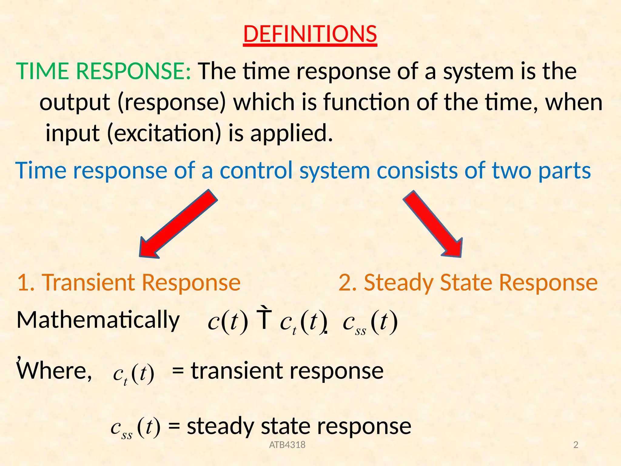
TIME RESPONSE: Thetime response of a system is the
output (response) which is function of the time, when
input (excitation) is applied.
Time response of a control system consists of two parts
1. Transient Response 2. Steady State Response
Mathematically
,
c(t) ct (t) css (t)
ATB4318 2
Where, ct (t) = transient response
css (t) = steady state response
3.
TRANSIENT RESPONSE: Thetransient response is the
part of response which goes to zero as time
increases. Mathematically
ATB4318 3
Limit ct (t)
0
t
The transient response may be exponential or
oscillatory in nature.
STEADY STATE: The steady state response is the part of
the total response after transient has died.
STEADY STATE ERROR: If the steady state response of
the output does not match with the input then the
system has steady state error, denoted by ess .
4.
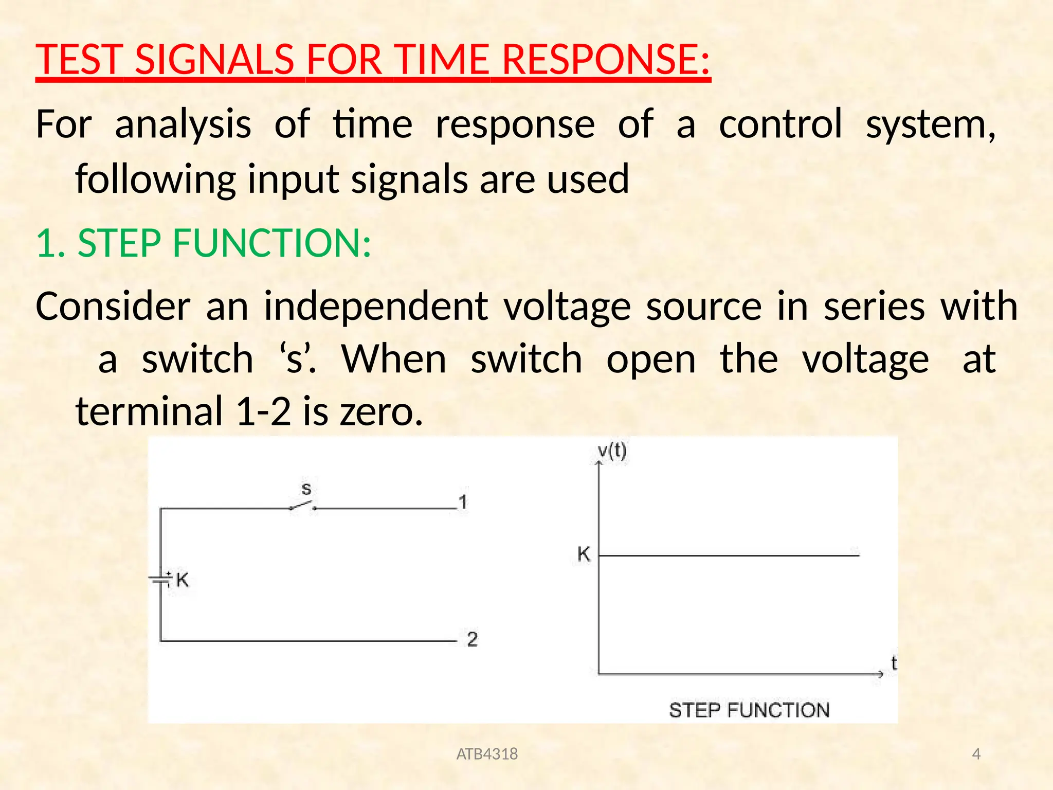
TEST SIGNALS FORTIME RESPONSE:
For analysis of time response of a control system,
following input signals are used
1. STEP FUNCTION:
Consider an independent voltage source in series with
a switch ‘s’. When switch open the voltage at
terminal 1-2 is zero.
ATB4318 4
5.
;
ATB4318 5
When theswitch is closed at t=0
;
Combining above two equations
;
;
A unit step function is denoted by u(t) and defined as
;
;
Mathematically
,
v(t) 0
t 0
v(t) K 0 t
v(t) 0
v(t)
K
t 0
0 t
u(t)
0
u(t)
1
t 0
0 t
6.
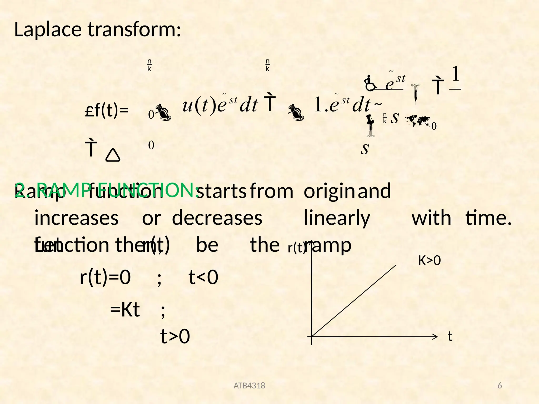
Laplace transform:
Ramp functionstartsfrom originand
increases or decreases linearly with time.
Let r(t) be the ramp
function then,
r(t)=0
=Kt
; t<0
;
t>0
0
0
2. RAMP FUNCTION:
1
s 0
s
est
£f(t)= u(t)est
dt 1.est
dt
K>0
ATB4318 6
t
r(t)
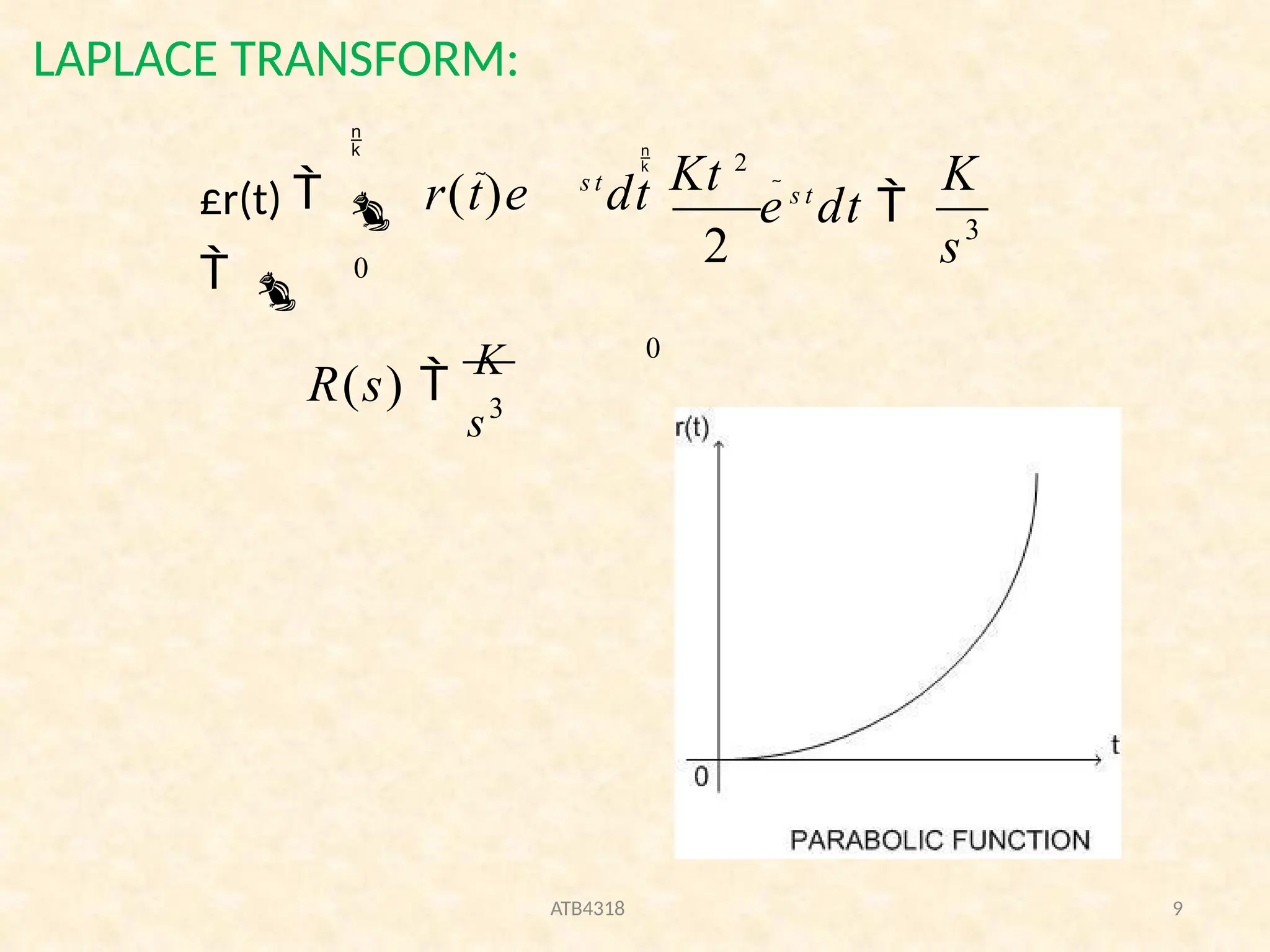
7.
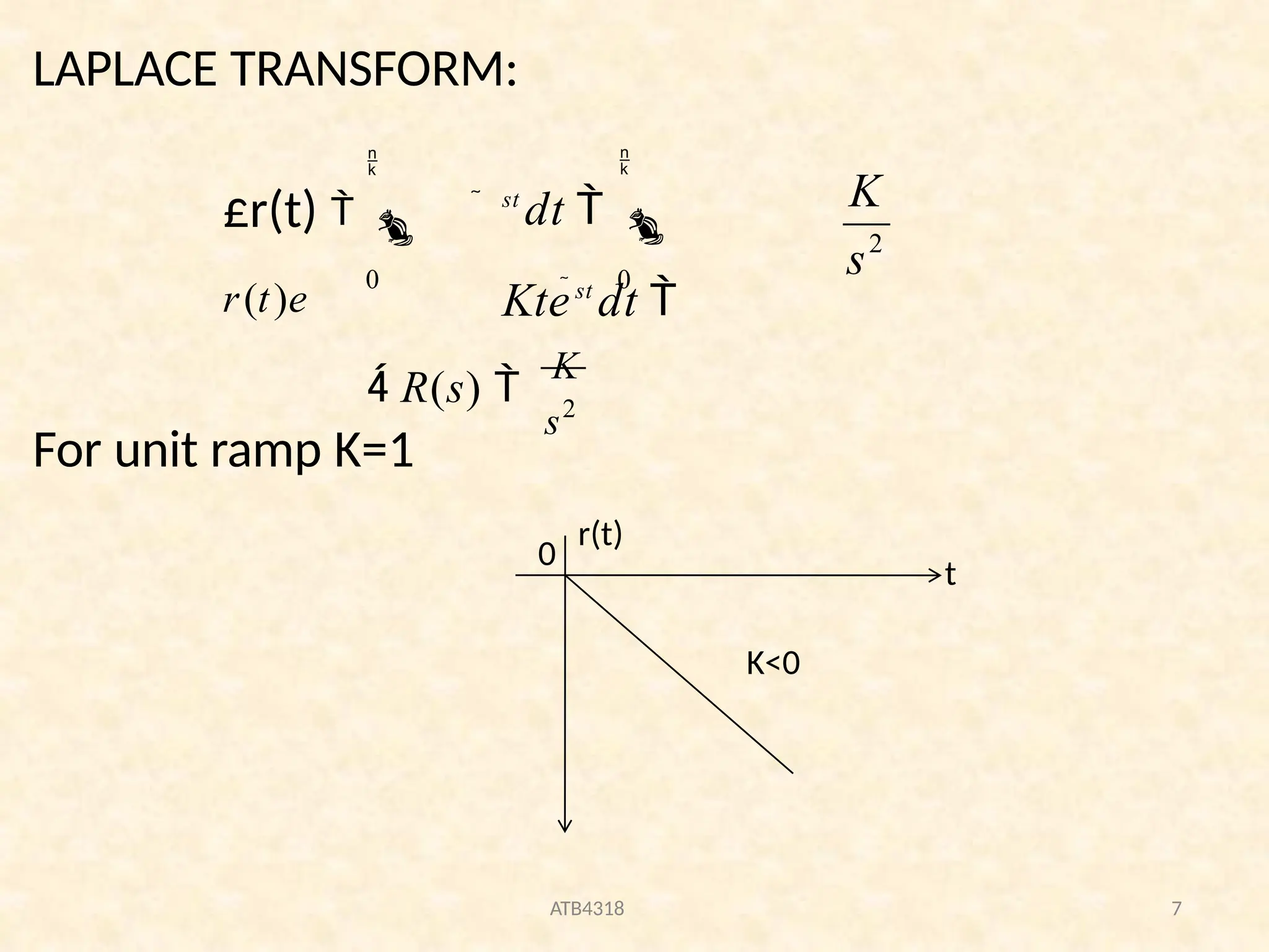
LAPLACE TRANSFORM:
For unitramp K=1
2
0
0
s
K
st
dt
Ktest
dt
£r(t)
r(t)e
s2
R(s)
K
t
ATB4318 7
r(t)
K<0
0
8.
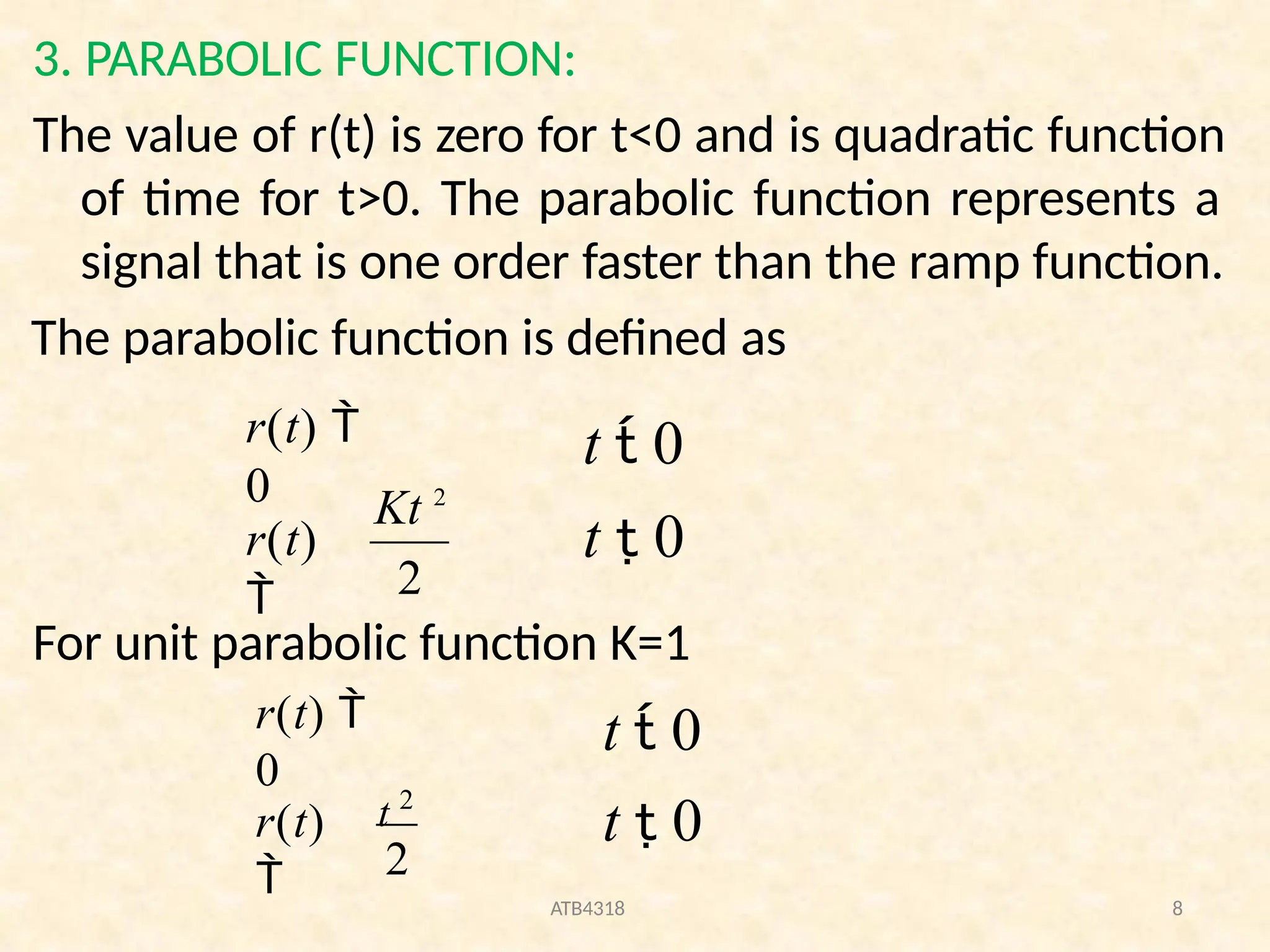
3. PARABOLIC FUNCTION:
Thevalue of r(t) is zero for t<0 and is quadratic function
of time for t>0. The parabolic function represents a
signal that is one order faster than the ramp function.
The parabolic function is defined as
For unit parabolic function K=1
2
Kt 2
r(t)
r(t)
0
t 0
t 0
2
ATB4318 8
t 2
r(t)
r(t)
0
t 0
t 0
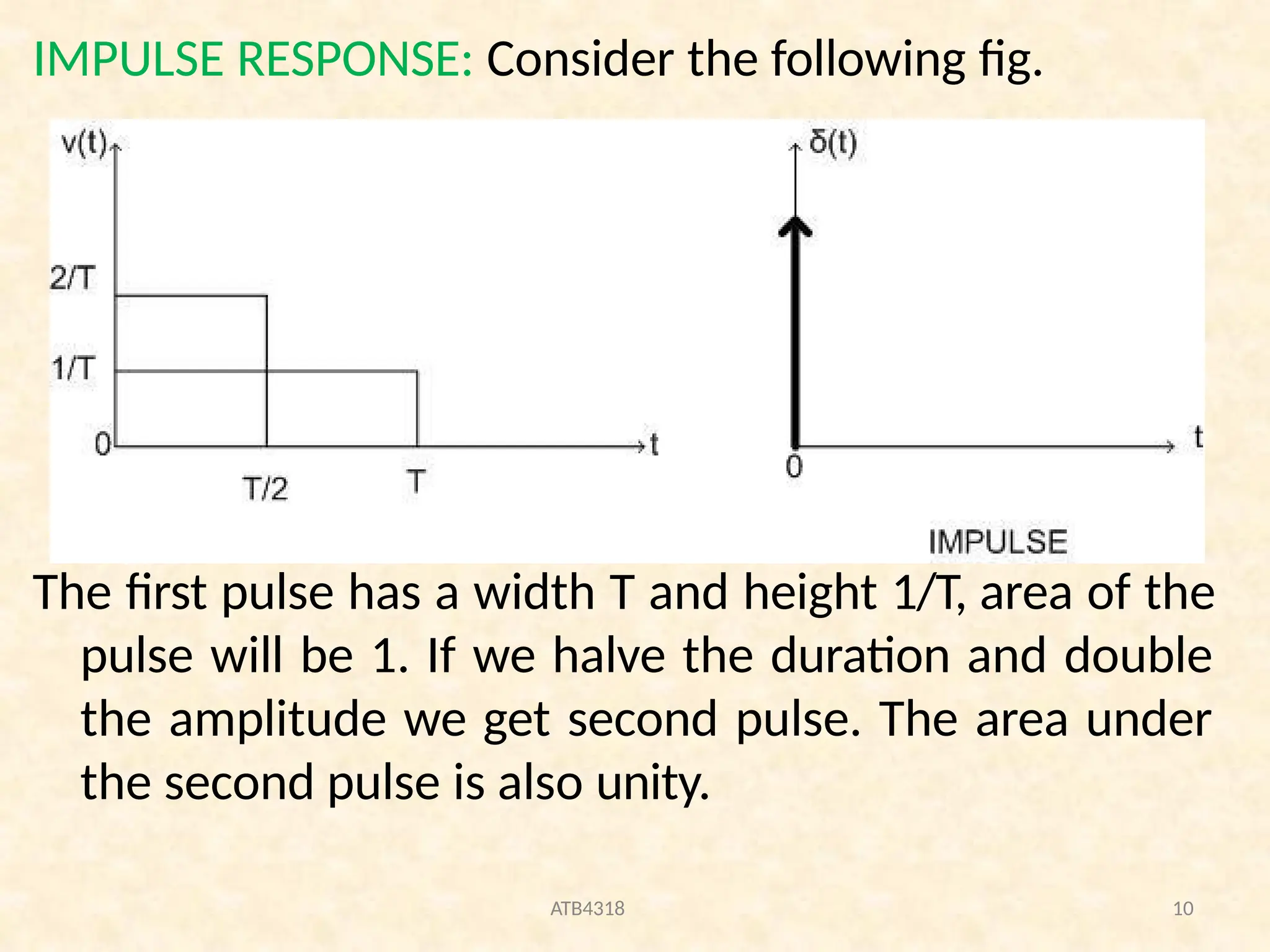
IMPULSE RESPONSE: Considerthe following fig.
The first pulse has a width T and height 1/T, area of the
pulse will be 1. If we halve the duration and double
the amplitude we get second pulse. The area under
the second pulse is also unity.
ATB4318 10
11.
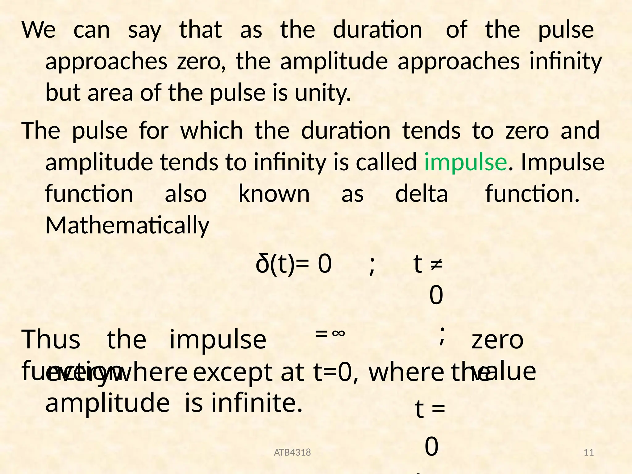
We can saythat as the duration of the pulse
approaches zero, the amplitude approaches infinity
but area of the pulse is unity.
The pulse for which the duration tends to zero and
amplitude tends to infinity is called impulse. Impulse
function also known as delta function.
Mathematically
ATB4318 11
Thus the impulse
function
δ(t)= 0 ; t ≠
0
=∞ ;
t =
0
zero
value
everywhereexcept at t=0, where the
amplitude is infinite.
12.
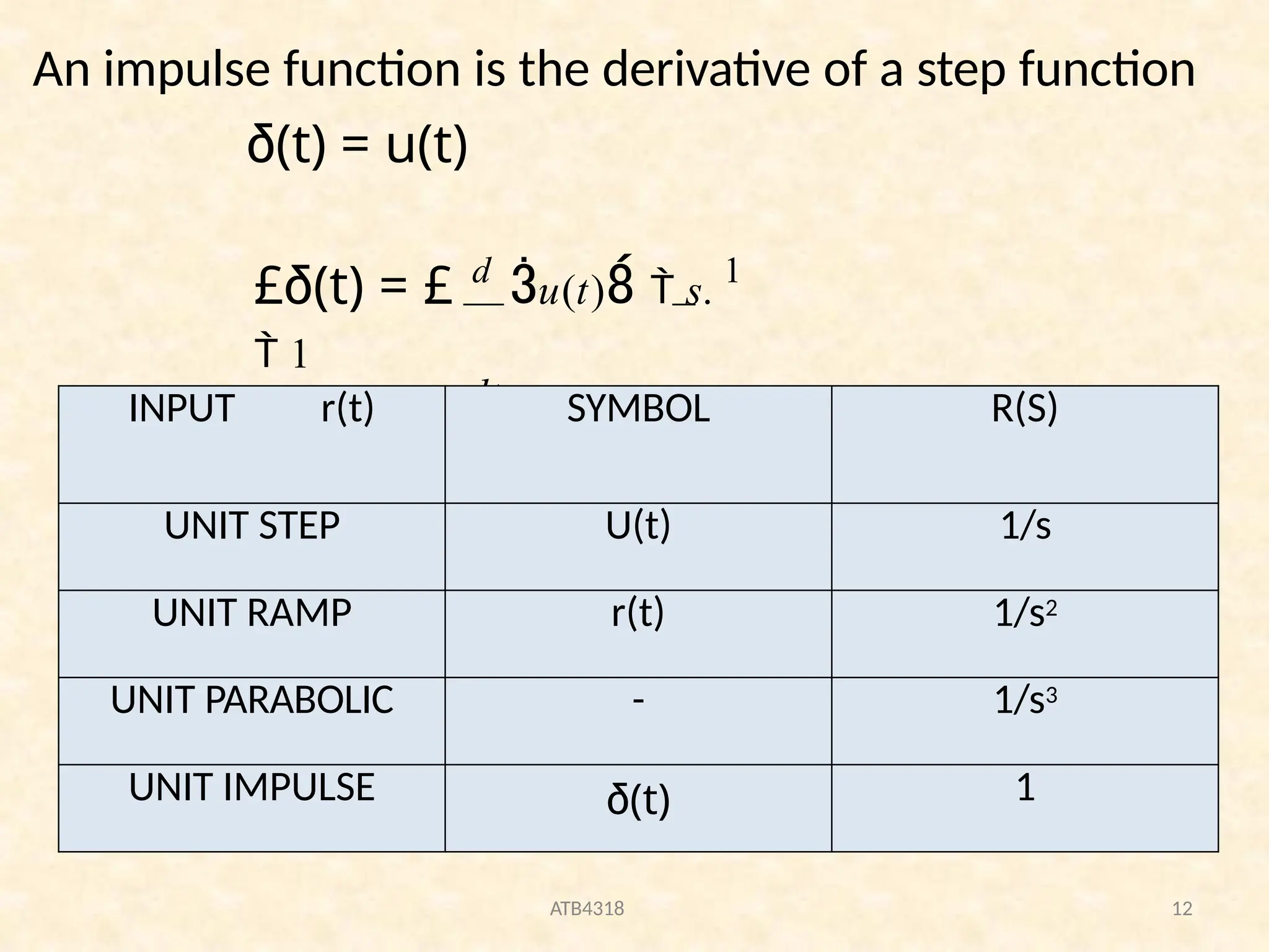
An impulse functionis the derivative of a step function
δ(t) = u(t)
£δ(t) = £ d
u(t) s.
1
1
dt
s
ATB4318 12
INPUT r(t) SYMBOL R(S)
UNIT STEP U(t) 1/s
UNIT RAMP r(t) 1/s2
UNIT PARABOLIC - 1/s3
UNIT IMPULSE δ(t) 1
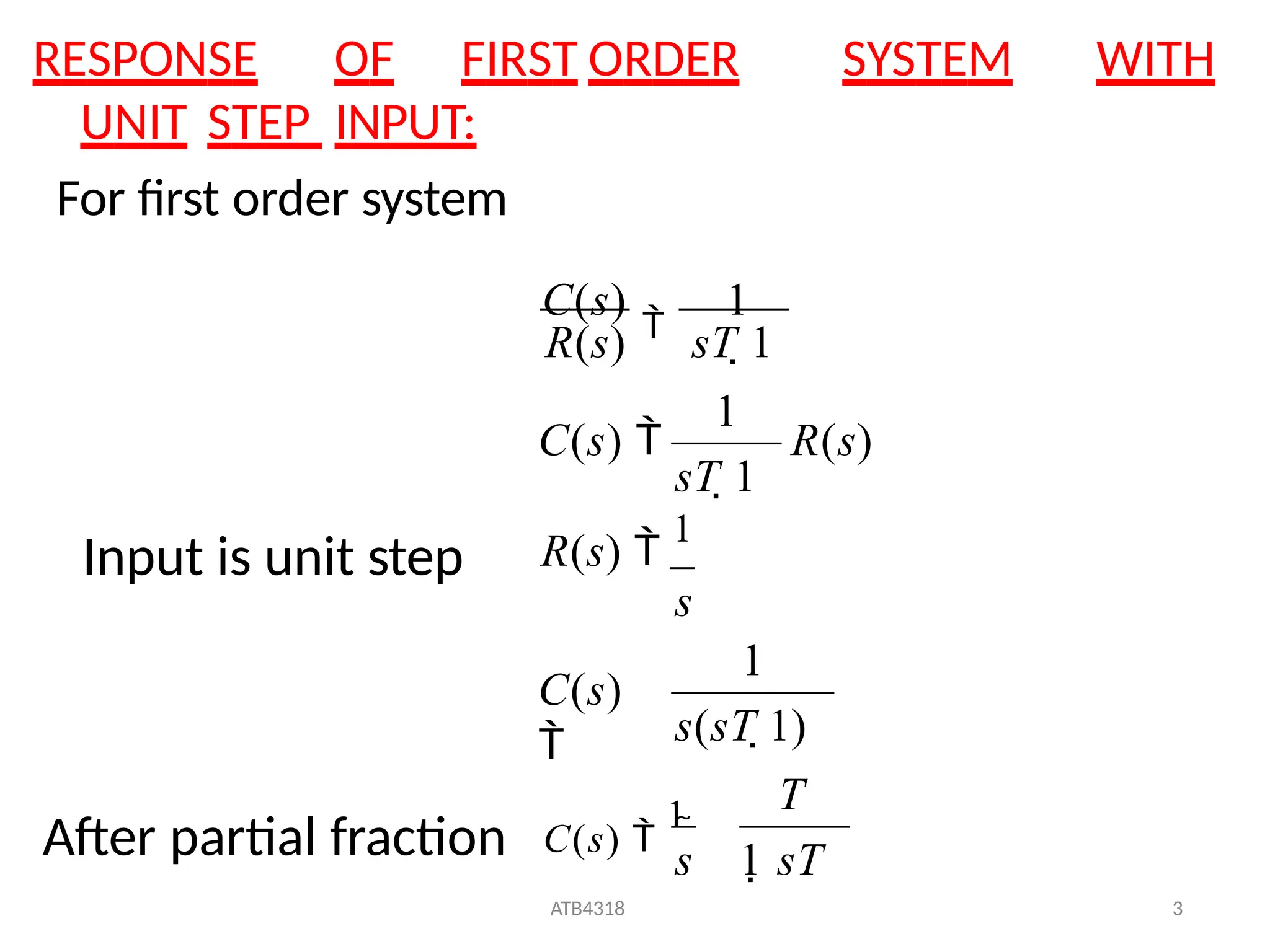
RESPONSE OF FIRSTORDER SYSTEM WITH
UNIT STEP INPUT:
For first order system
s 1 sT
ATB4318 3
T
After partial fraction C(s)
1
s(sT 1)
C(s)
R(s)
1
s
R(s)
sT 1
C(s)
1
1
1
R(s) sT 1
C(s)
Input is unit step
15.
ATB4318 4
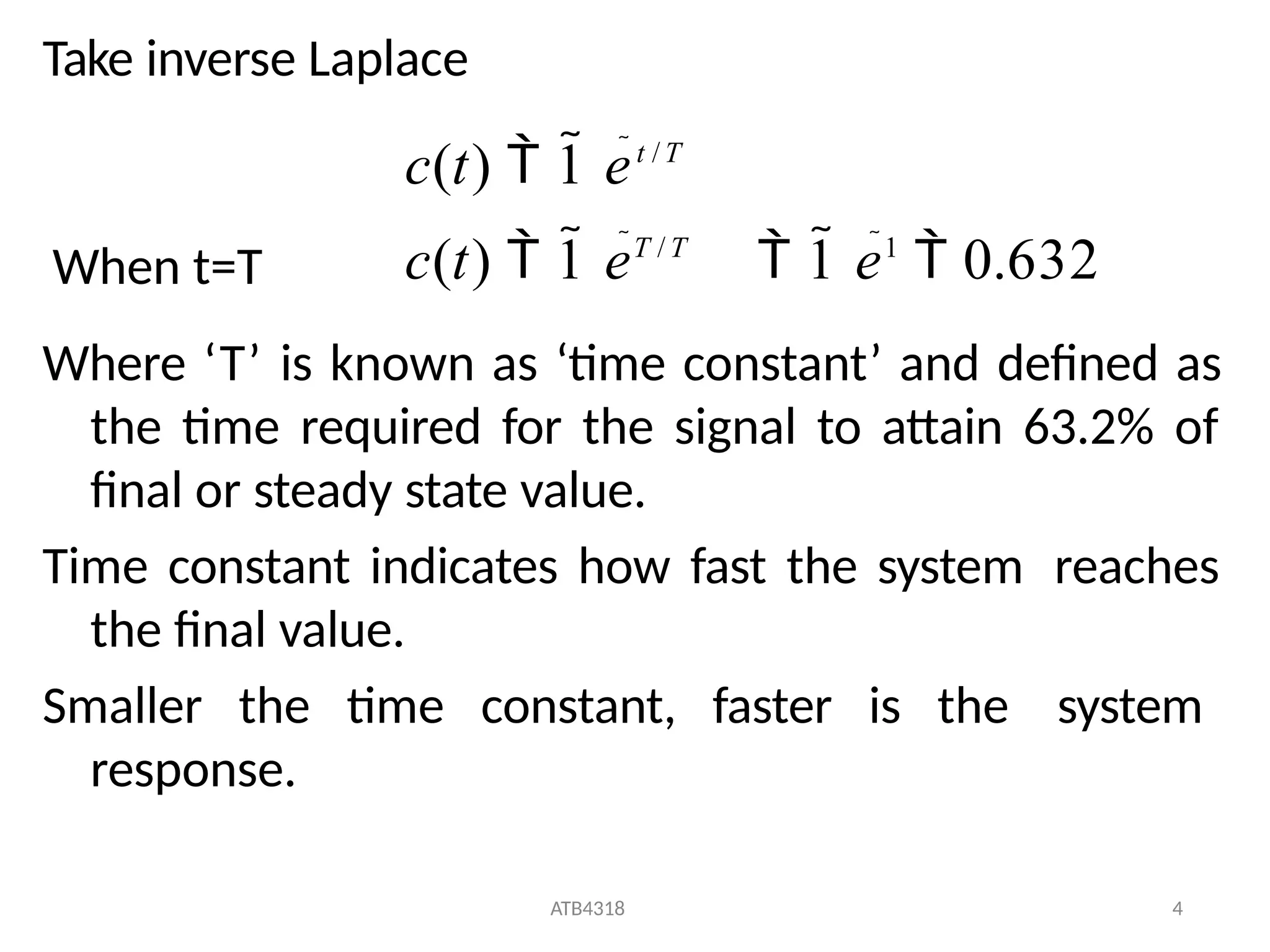
Take inverseLaplace
Where ‘T’ is known as ‘time constant’ and defined as
the time required for the signal to attain 63.2% of
final or steady state value.
Time constant indicates how fast the system reaches
the final value.
Smaller the time constant, faster is the system
response.
c(t) 1 eT / T
1 e1
0.632
c(t) 1 et / T
When t=T
16.
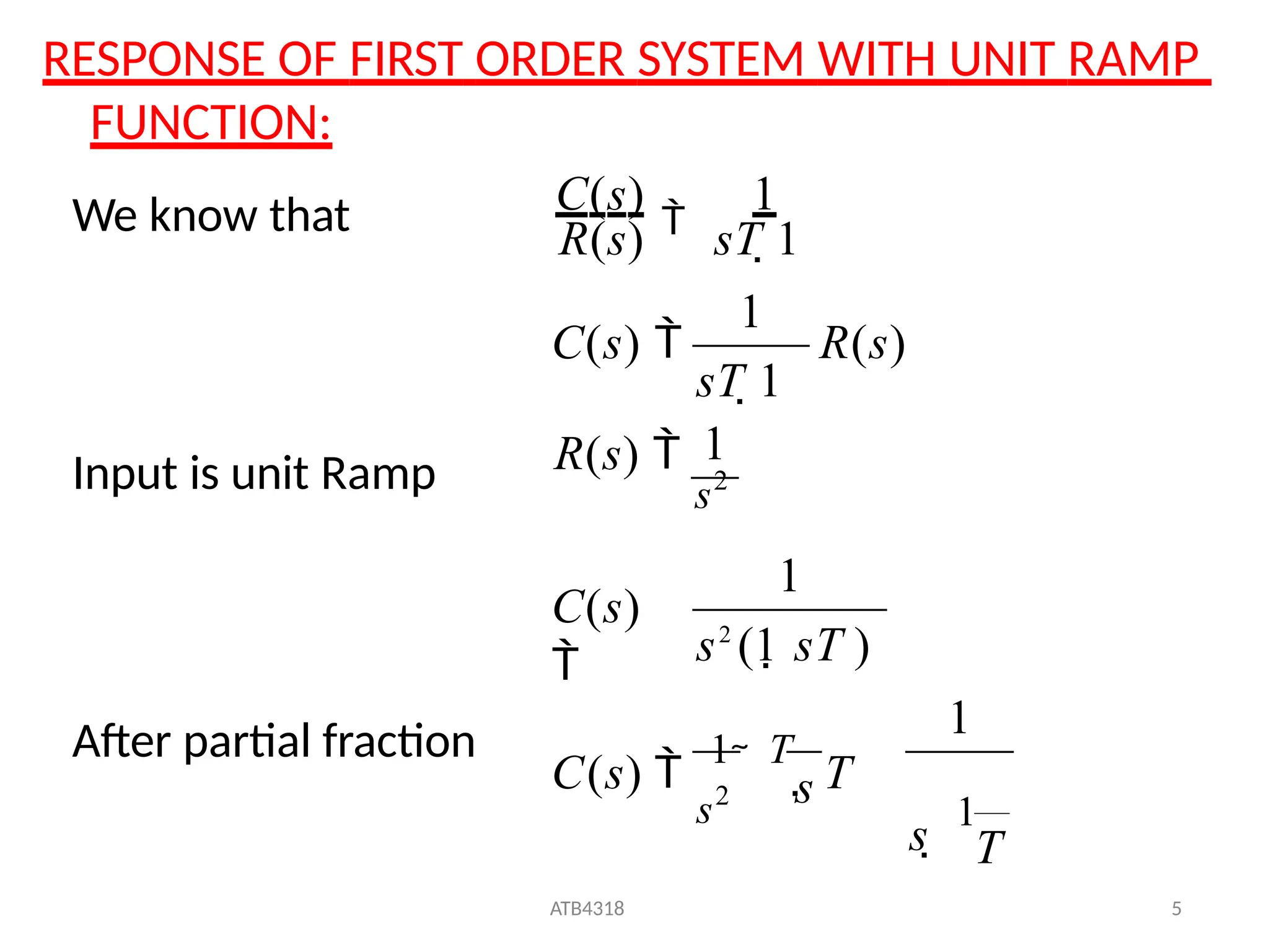
RESPONSE OF FIRSTORDER SYSTEM WITH UNIT RAMP
FUNCTION:
T
ATB4318 5
s
1
s
s2
C(s)
1
T
T
s2
(1 sT )
C(s)
R(s)
C(s)
1
1
1
1
R(s)
s2
1
sT 1
R(s) sT 1
C(s)
Input is unit Ramp
After partial fraction
We know that
17.
ATB4318 6
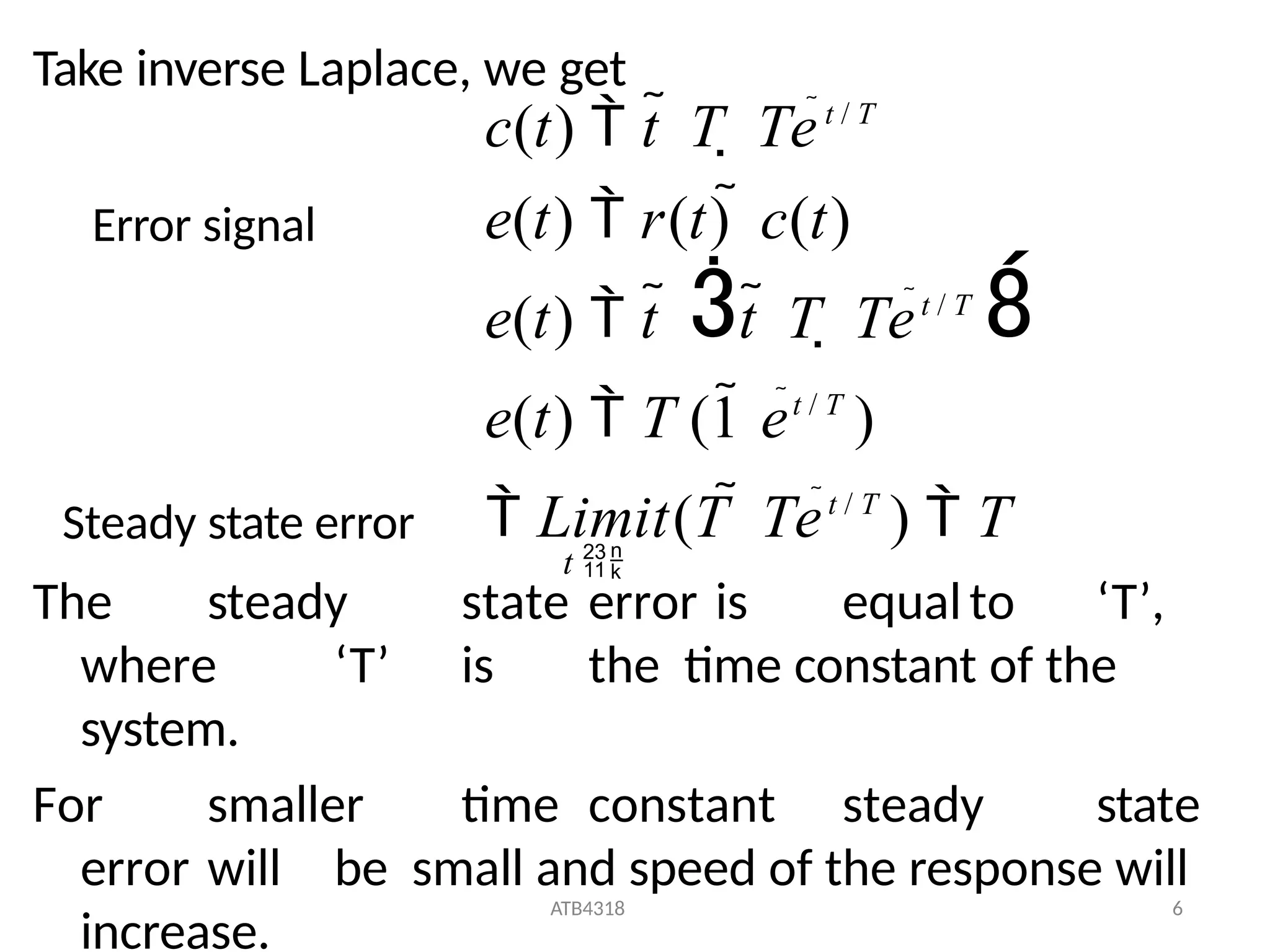
Take inverseLaplace, we get
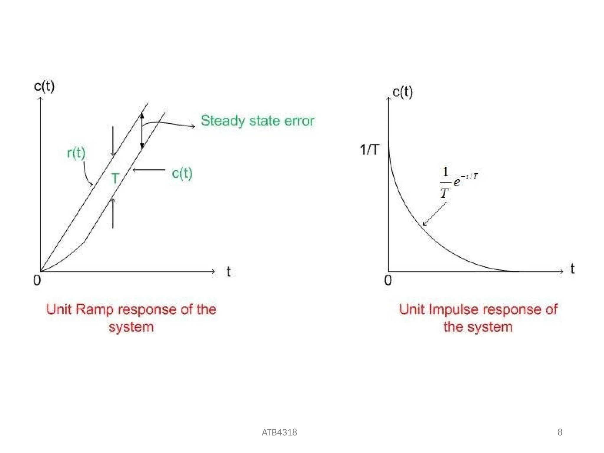
The steady state error is equalto ‘T’,
where ‘T’ is the time constant of the
system.
For smaller time constant steady state
error will be small and speed of the response will
increase.
c(t) t T Tet / T
t
e(t) r(t) c(t)
e(t) t t T Tet / T
e(t) T (1 et / T
)
Limit(T Tet / T
) T
Error signal
Steady state error
18.
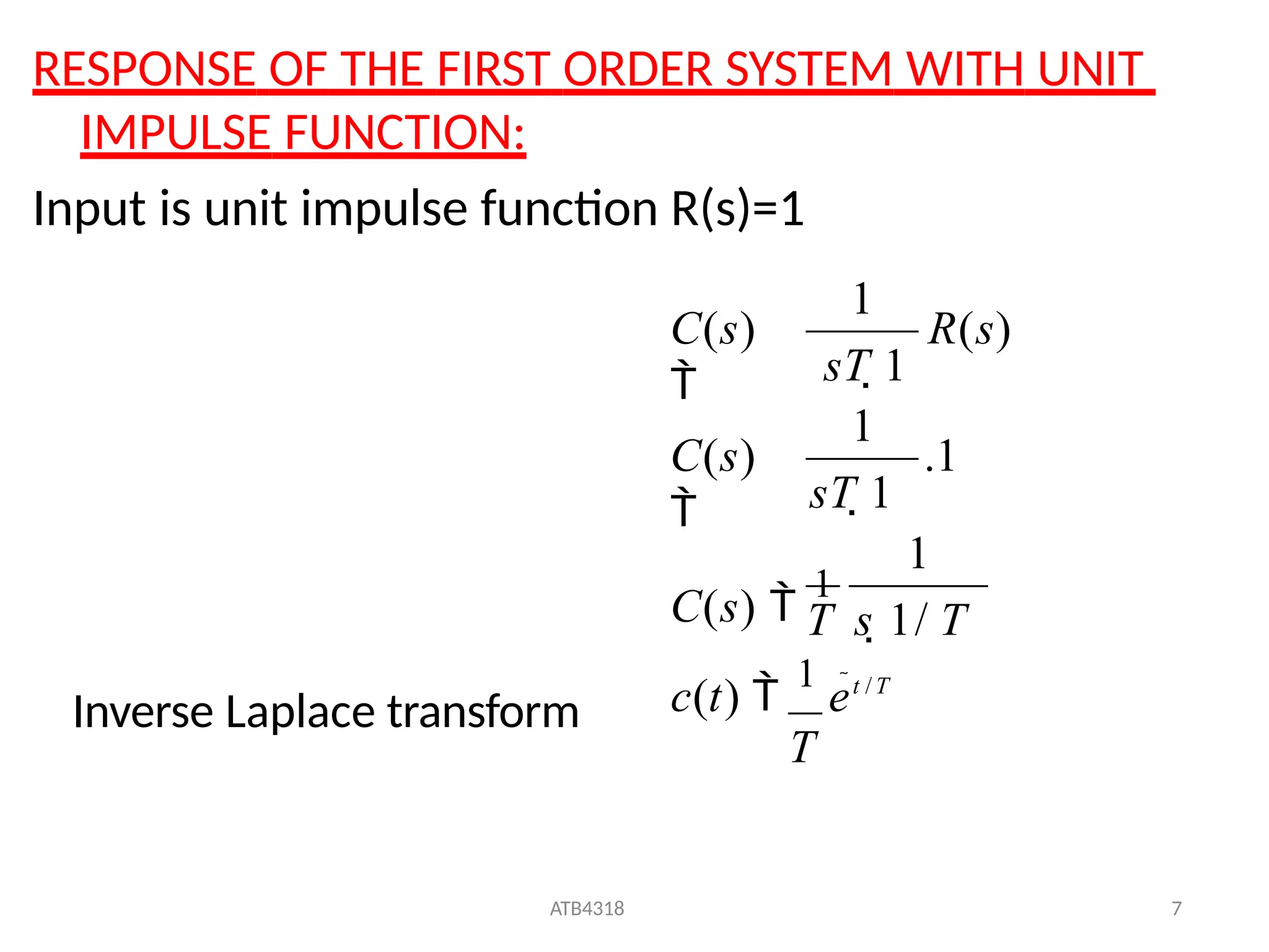
RESPONSE OF THEFIRST ORDER SYSTEM WITH UNIT
IMPULSE FUNCTION:
Input is unit impulse function R(s)=1
c(t)
1
et / T
T
ATB4318 7
T s 1/ T
C(s)
1
C(s)
R(s)
C(s)
1
.1
sT 1
sT 1
1
1
Inverse Laplace transform
R(s)
1
s
R(s)
1
s2
R(s)
1
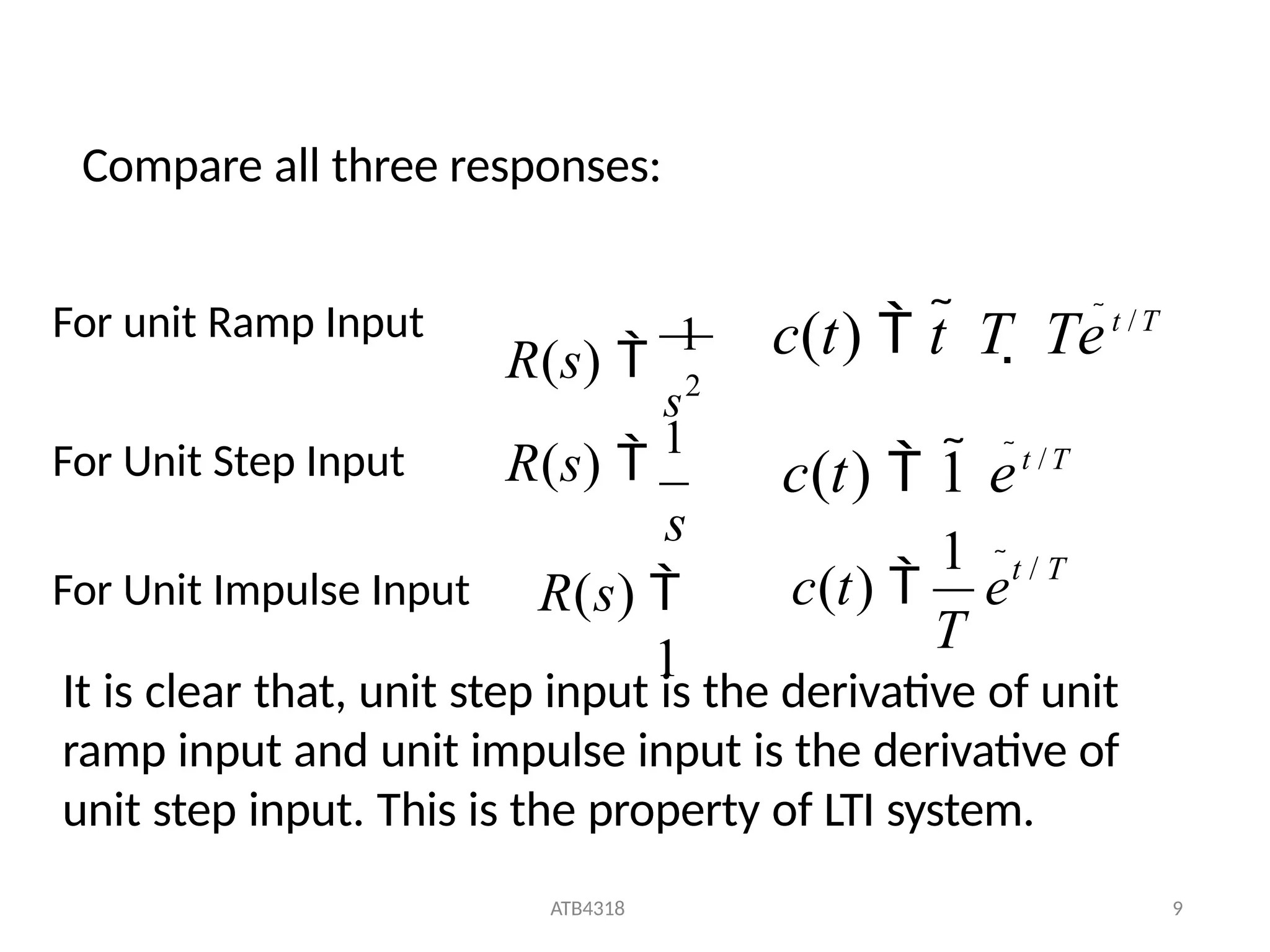
For unit Ramp Input
For Unit Step Input
For Unit Impulse Input
c(t) t T Tet /T
c(t) 1 et /T
T
ATB4318 9
1 t / T
c(t) e
It is clear that, unit step input is the derivative of unit
ramp input and unit impulse input is the derivative of
unit step input. This is the property of LTI system.
Compare all three responses:
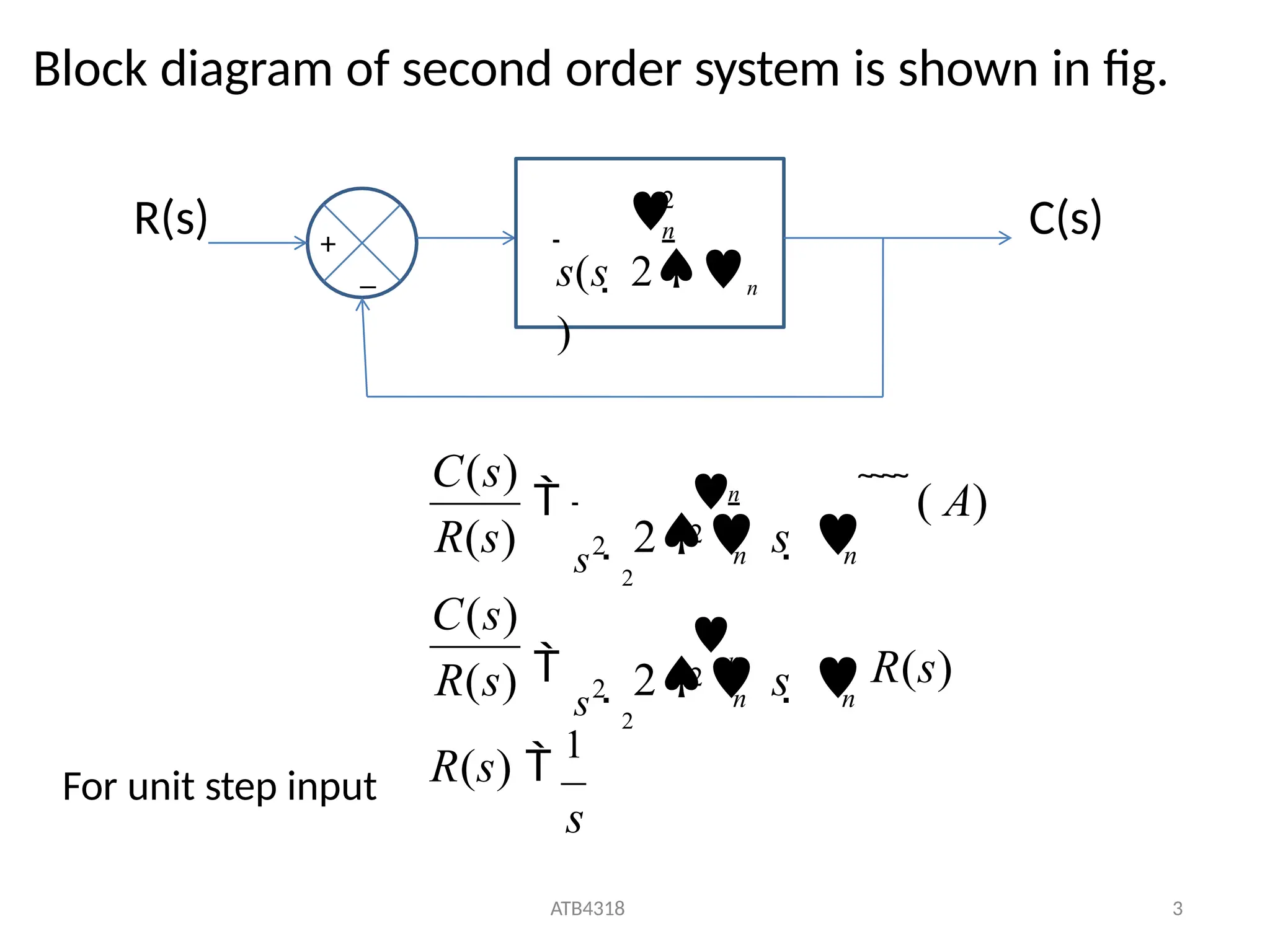
Block diagram ofsecond order system is shown in fig.
R(s) C(s)
_
+
2
n
s(s 2n
)
R(s)
1
s
ATB4318 3
R(s)
R(s)
C(s)
C(s)
n
n
n n
s2
s2
n
R(s)
n
( A)
2 s
2
2
2 s
2
2
For unit step input
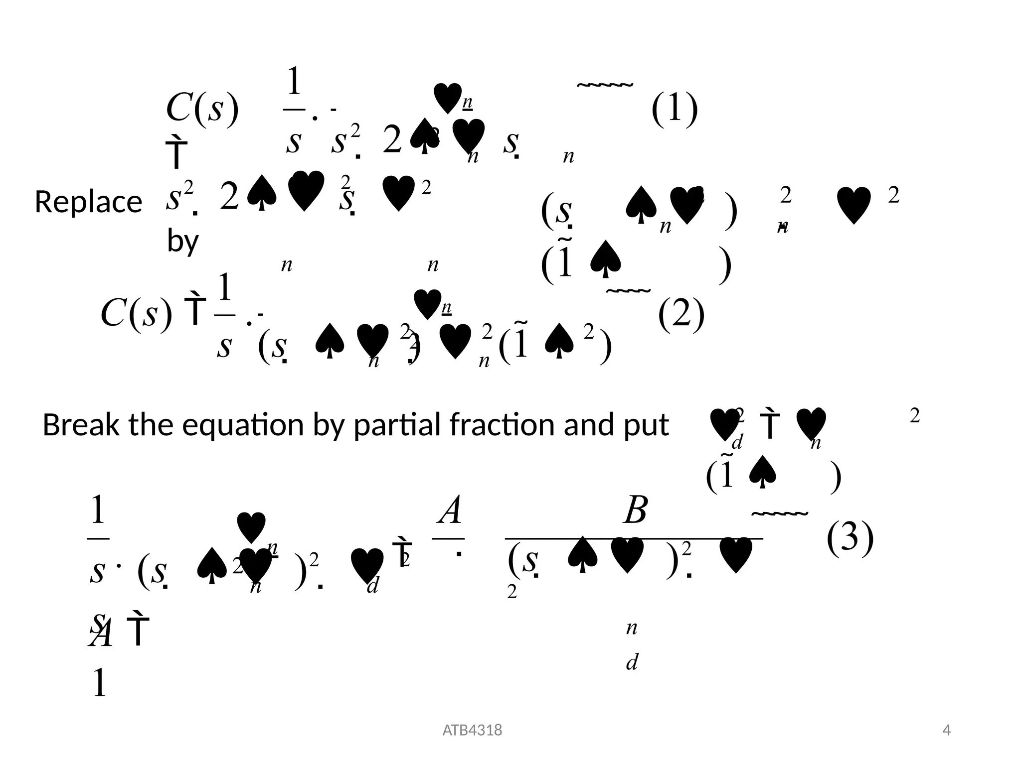
23.
s2
2 s 2
by
n n
1
C(s)
n
n
2
. n
(1)
s s2
2 s
2
Replace 2 2 2
n n
(s )
(1 )
Break the equation by partial fraction and put 2 2
2
(1 )
n
d
A
1
(3)
(s )2
2
n
d
1
A B
n d
. n
s (s )2
2
s
2
1
ATB4318 4
2 2 2
2
n n
s (s ) (1 )
C(s) . n
(2)
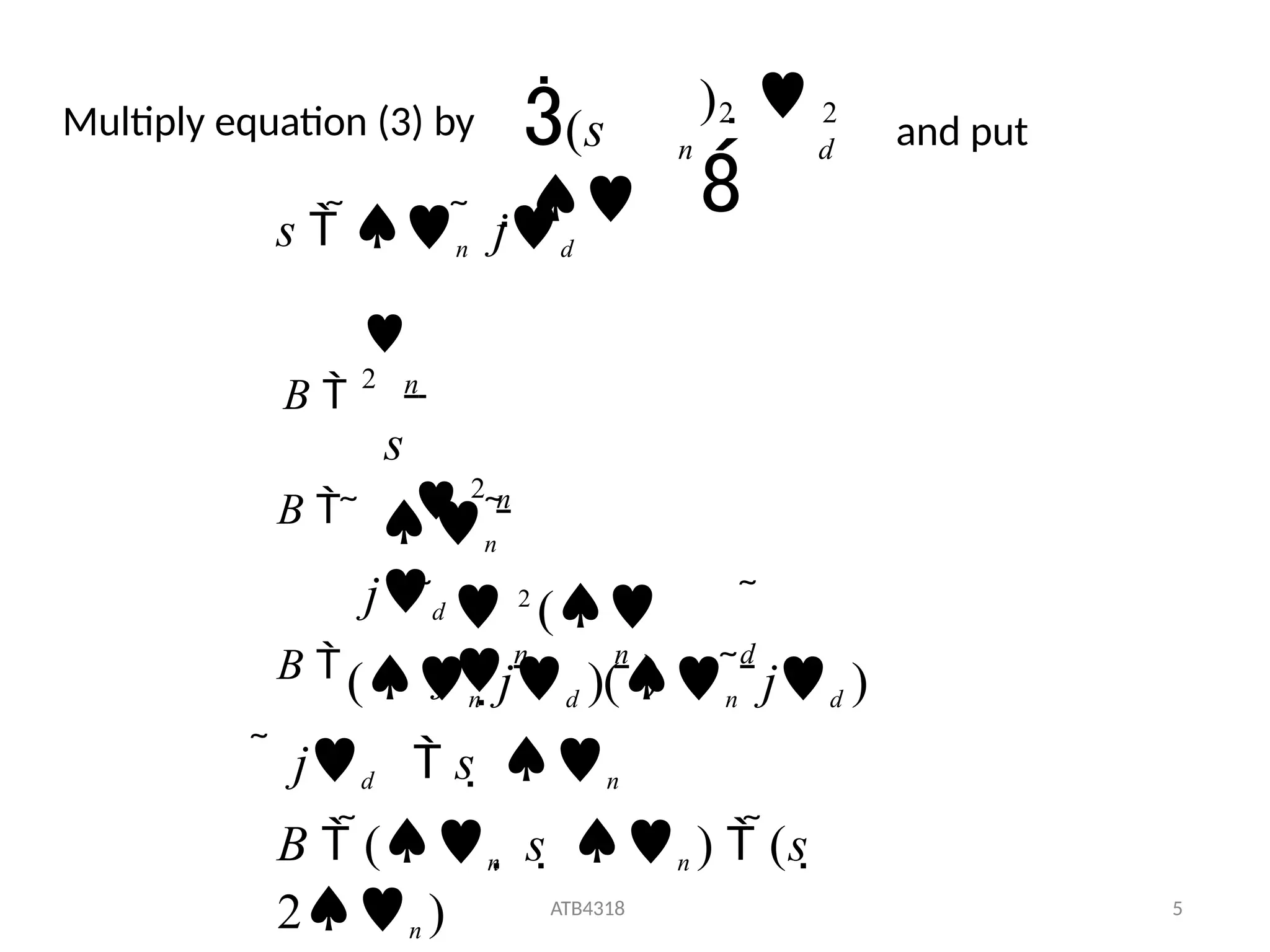
24.
ATB4318 5
2
2
d
)
n
(s
Multiplyequation (3) by and put
(n jd )(n jd )
jd s n
B (n s n ) (s
2n )
2
(
j )
2
B n n d
n
jd
B n
s n jd
B n
s
2
25.
Equation (1) canbe written as
n
.
2
2
2 2
2
2
(4)
d
s
n
n
n
(s )
d
d
n d
d
n
s (s )
C(s)
1
s
n
s
C(s)
1
(s )
Laplace Inverse of equation (4)
(5)
d
c(t) 1 e
d
n
d
n
e .sin
t
t
n
.cos t
t
d n 1
2
ATB4318 6
Put
26.
e
nt
c(t) 1
d
sindt
.sint
1 2
.cos t
d
d
n
c(t) 1 e
t
1
2
1 2
cos t
sin(d t
)
ATB4318 7
1
2
c(t) 1
1
2
tan
1 2
sin
cos
e
nt
Put
27.
1
2
c(t) 1
sin(
en
t
1 2
1 2
)t tan 1
(6)
n
Put the values of d &
e(t)
ATB4318 8
Error signal for the system
e(t) r(t) c(t)
sin(
1
2
e
n t
1 2
1 2
)t tan 1
(7)
n
t
The steady state value of c(t)
ess Limit c(t) 1
28.
Therefore at steadystate there is no
error between input and output.
= natural frequency of oscillation or undamped
natural frequency.
= damping factor or actual damping or
n
d = damped frequency of
oscillation.
n
damping coefficient.
For equation (A) two poles (for 0 1 )
are
j
1
2
n n
ATB4318 9
29.
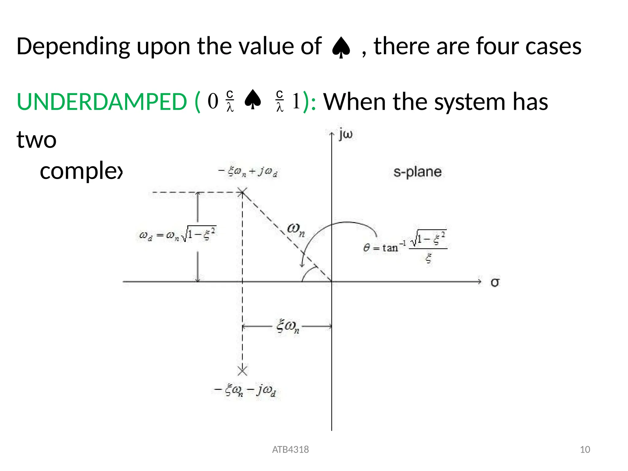
Depending upon thevalue of , there are four cases
UNDERDAMPED ( 0 1): When the system has
two
complex conjugate poles.
ATB4318 10
30.
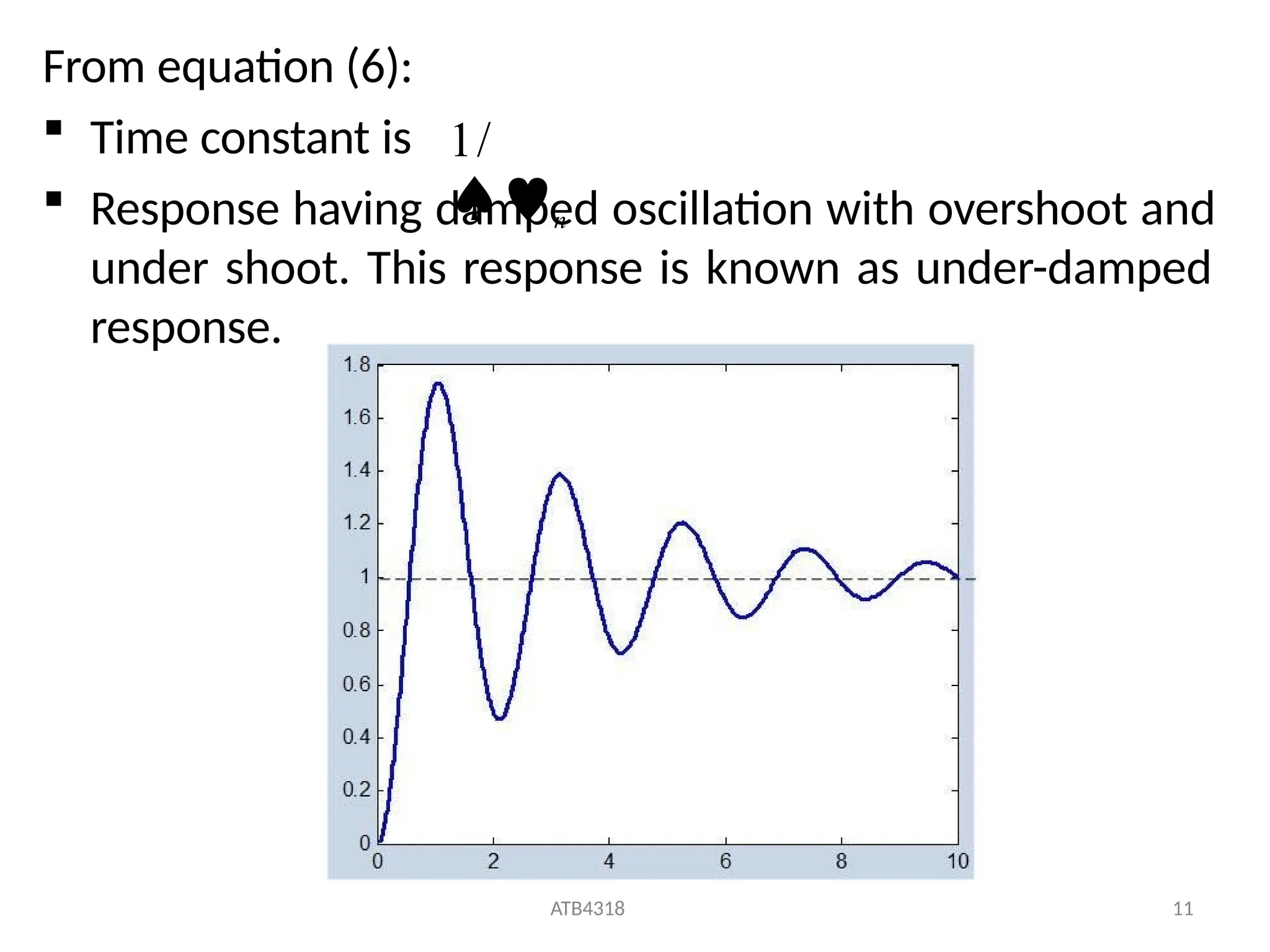
From equation (6):
Time constant is
Response having damped oscillation with overshoot and
under shoot. This response is known as under-damped
response.
1/
n
ATB4318 11
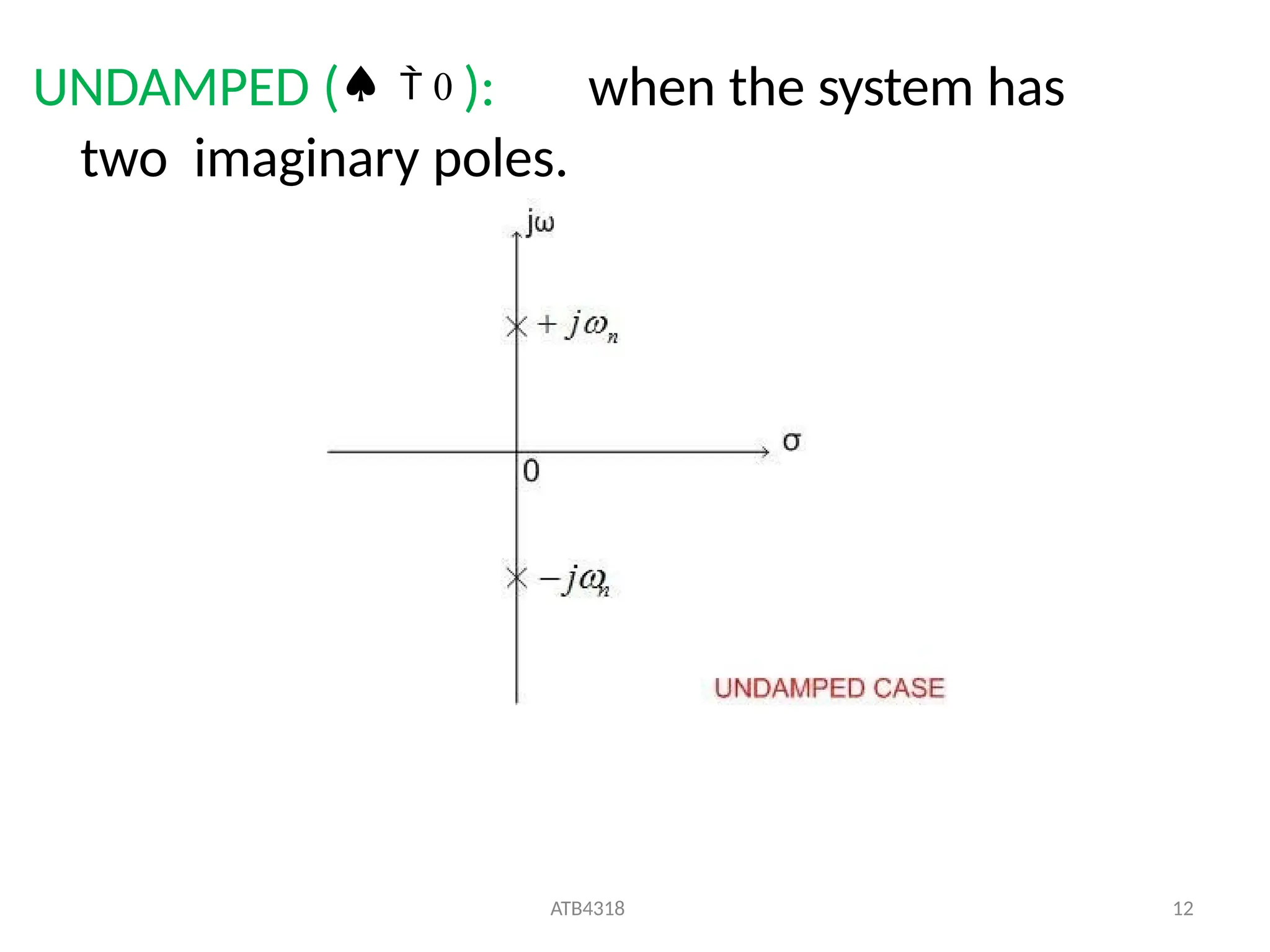
31.
UNDAMPED ( 0 ): when the system has
two imaginary poles.
ATB4318 12
32.
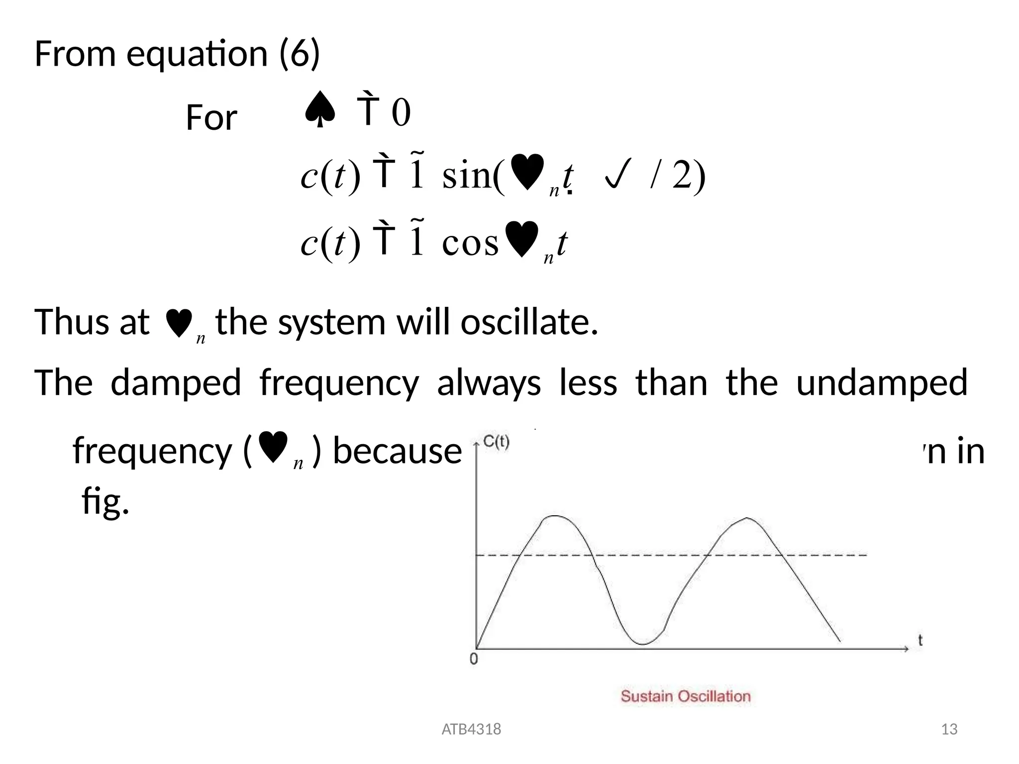
From equation (6)
For 0
c(t) 1 sin(nt / 2)
c(t) 1 cosnt
Thus at n the system will oscillate.
The damped frequency always less than the undamped
frequency (n ) because of . The response is shown in
fig.
ATB4318 13
33.
CRITICALLY DAMPED ( 1): When the system has
two real and equal poles. Location of poles for
critically damped is shown in fig.
ATB4318 14
34.
1
ATB4318 15
1
C(s)
n
n
n
n
nn
. n
2
2
s(s )2
C(s) n
s s2
2s
2
2 n
s (s )2
n
1
1
s(s )2
s
For
After partial
fraction
Take the inverse Laplace
c(t) 1 ent
t ent
n
c(t) 1 ent
(1
t) (8)
n
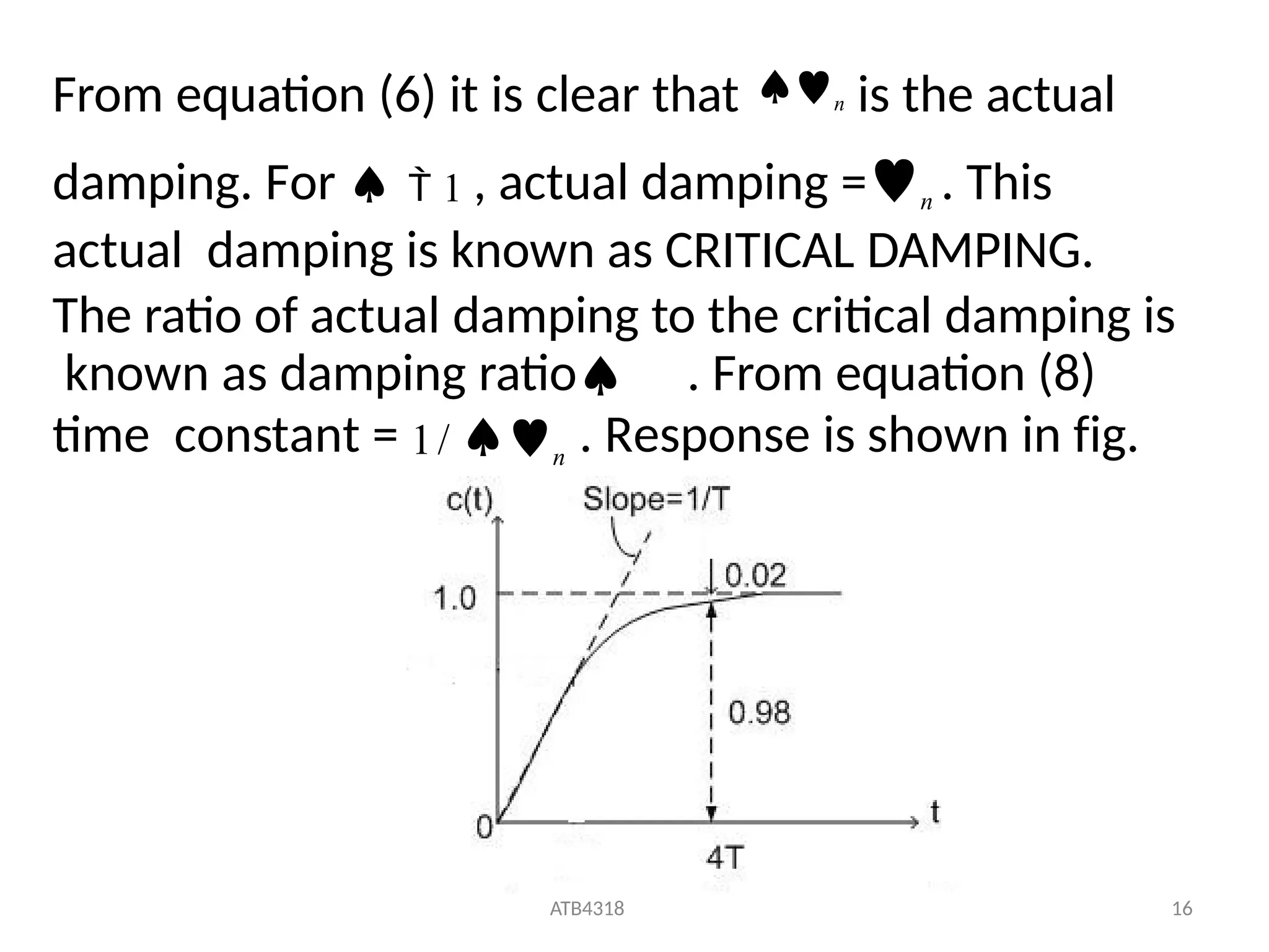
35.
From equation (6)it is clear that n is the actual
damping. For 1 , actual damping =n . This
actual damping is known as CRITICAL DAMPING.
The ratio of actual damping to the critical damping is
known as damping ratio . From equation (8)
time constant = 1/ n
. Response is shown in fig.
ATB4318 16
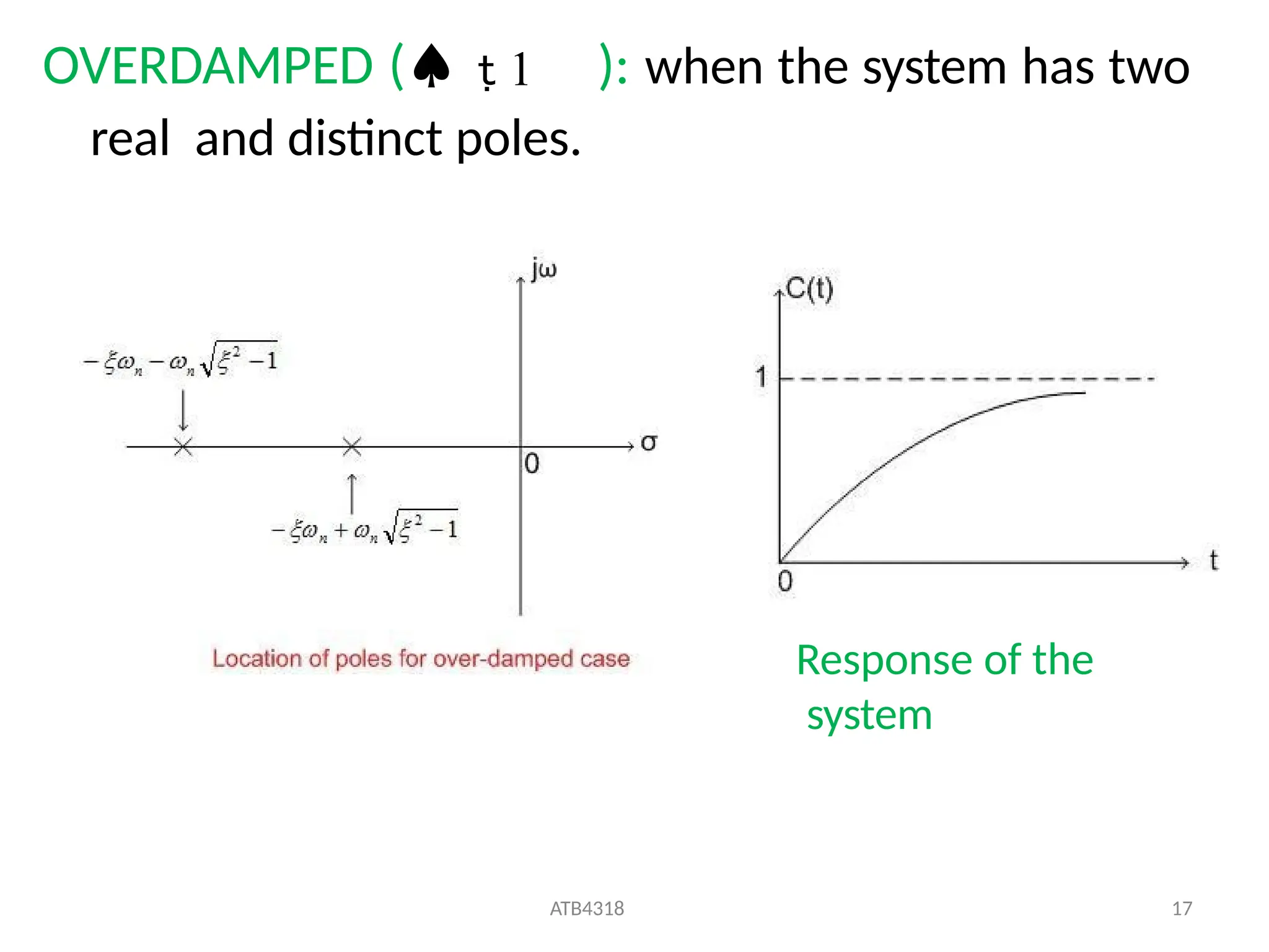
36.
OVERDAMPED ( 1 ): when the system has two
real and distinct poles.
Response of the
system
ATB4318 17
37.
From equation (2)
1
22 2
2
n
n
s (s ) (1)
C(s) . n
(9)
2
2
( 1)
2
n
d
Put
1
ATB4318 18
2 2
d
n
C(s) . n
(10)
s (s )
2
We get
C(s) n
(11)
s(s n d )(s n
d )
Equation (10) can be written as
2
38.
After partial fractionof equation (11) we get
Put the value of
d
(12)
1
1
C(s)
1
s
2
2
1
d
n
1
s
2 2
1
n d
s
2 2
1
1
ATB4318 19
2
2
2
(13)
1)
1)
2 1
2
2
1
2 2
1
n n
1s n n (
1 s
(
C(s)
1
s
39.
Inverse Laplace ofequation (13)
From equation (14) we get two time constants
(14)
2
e( 2
1)nt
2
2 2
1( 1) 2 2
1( 1)
e( 2
1)nt
c(t) 1
n
ATB4318 20
n
1
2
2
1
( 1)
1)
(
2
T
1
T
40.
(15)
c(t) 1
2
2 2
1( 1)
e( 2
1)nt
From equation (14) it is clear that when is greater than
one there are two exponential terms, first term has time
constant T1 and second term has a time constant T2 . T1 <
T2 . In other words we can say that first exponential term
decaying much faster than the other exponential term.
So for time response we neglect it, then
(16)
ATB4318 21
1
2
T
n
( 2
1)
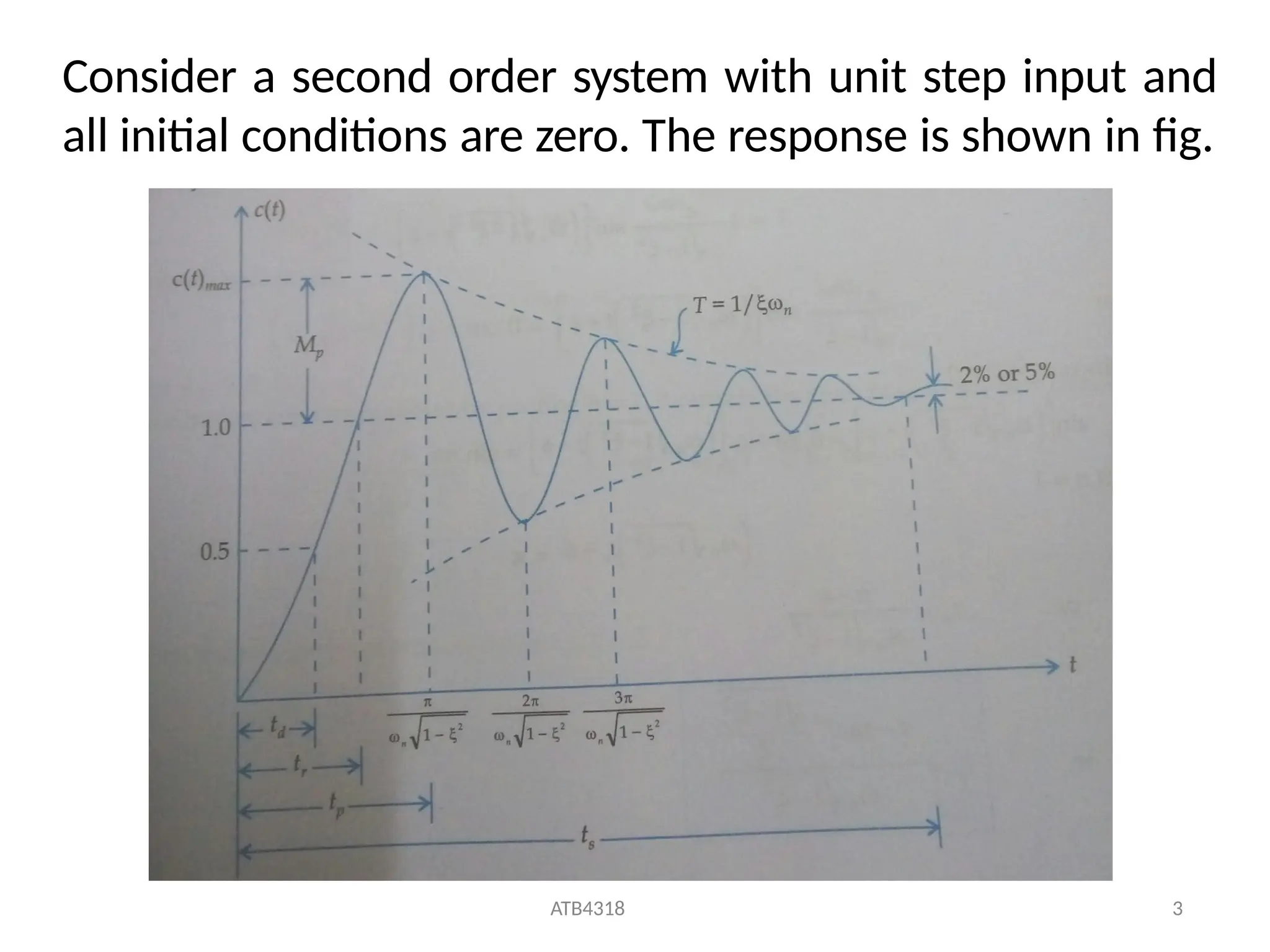
Consider a secondorder system with unit step input and
all initial conditions are zero. The response is shown in fig.
ATB4318 3
43.
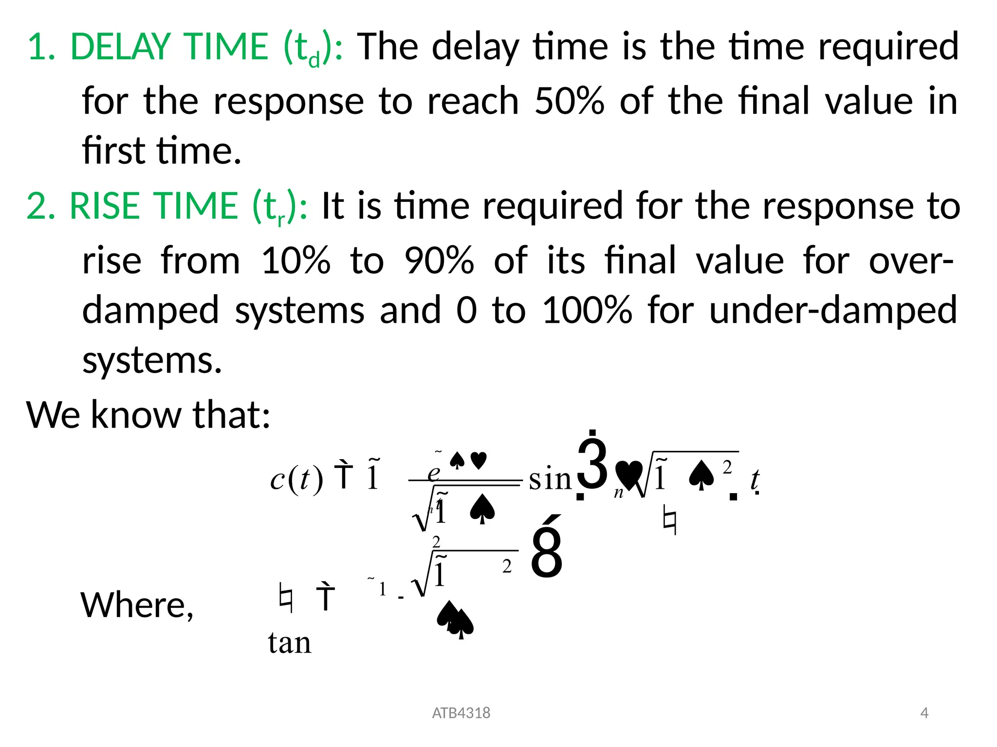
1. DELAY TIME(td): The delay time is the time required
for the response to reach 50% of the final value in
first time.
2. RISE TIME (tr): It is time required for the response to
rise from 10% to 90% of its final value for over-
damped systems and 0 to 100% for under-damped
systems.
We know that:
c(t) 1
tan
ATB4318 4
1
2
e
n t
2
1
1
2
sin
1 t
n
Where,
44.
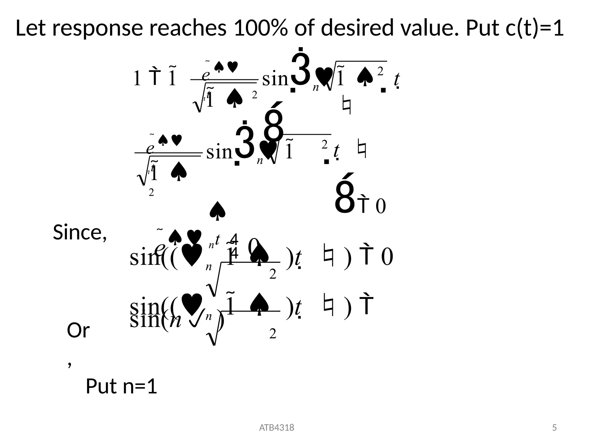
Let response reaches100% of desired value. Put c(t)=1
t
0
1 1
2
2
1
2
sin
1 2
sin 1
1 t
n
n
e
nt
e
nt
e nt
0
Since,
sin((n 1 )t ) 0
2
sin((n 1 )t )
sin(n ) 2
ATB4318 5
Or
,
Put n=1
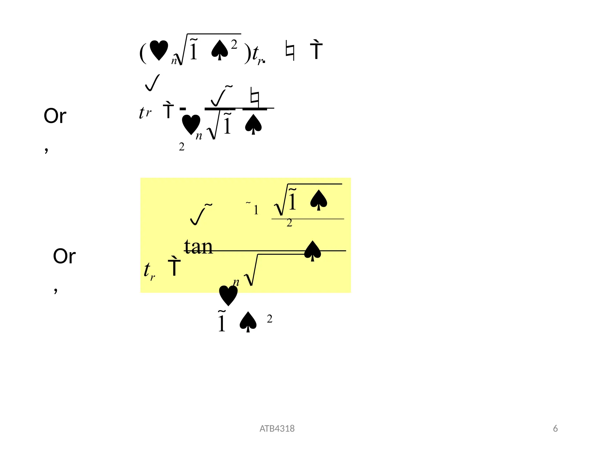
45.
1
2
2
r
(n1 )t
t
n
r
tan
ATB4318 6
1
n
1
2
tr
1 2
Or
,
Or
,
46.
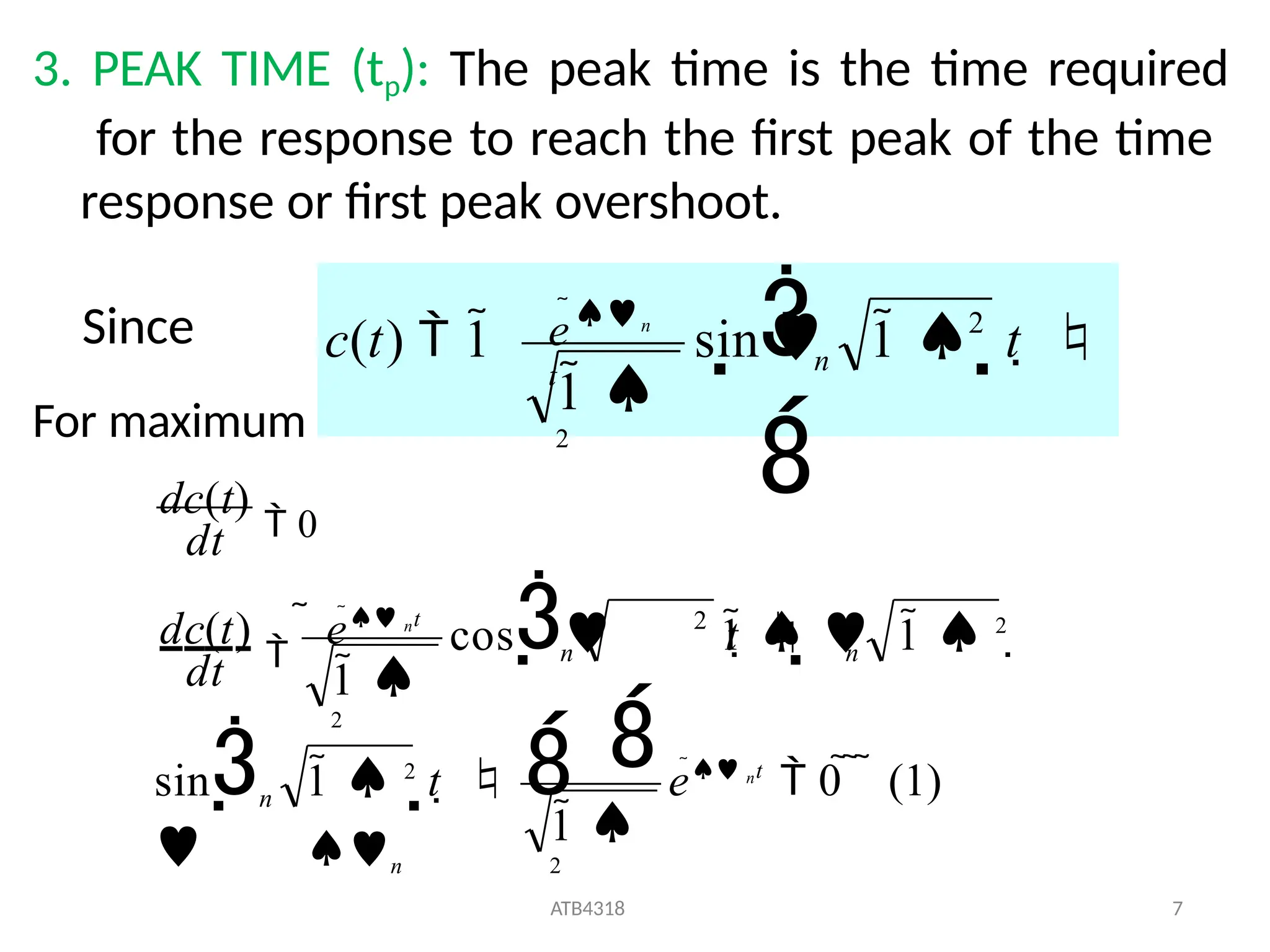
3. PEAK TIME(tp): The peak time is the time required
for the response to reach the first peak of the time
response or first peak overshoot.
Since
For maximum
t
n
en
t
2
1
1
2
c(t) 1 sin
e nt
0 (1)
ATB4318 7
1
2
1 2
t
n
1
2
dc(t)
0
dt
dc(t)
e nt 2
n
n
n t 1 2
cos 1
dt
sin
47.
Since,
Equation can bewritten as
e nt
0
cos1 2
t 1 2
sin
1 2
t
1 2
sin
n
n
Put and
cos
Equation (2) becomes
cos 1 2
t sin sin 1 2
t
cos
n n
sin
cos
ATB4318 8
cos(( 1 2
)t
)
sin(( 1 2
)t )
n
n
48.
(n 1 )t
n 2
p
tan((n 1 )t )
n 2
The time to various
peak
Where n=1,2,3,
…….
Peak time to first overshoot, put n=1
1
2
n
p
t
First minimum (undershoot) occurs at n=2
min
ATB4318 9
2
1
2
n
t
49.
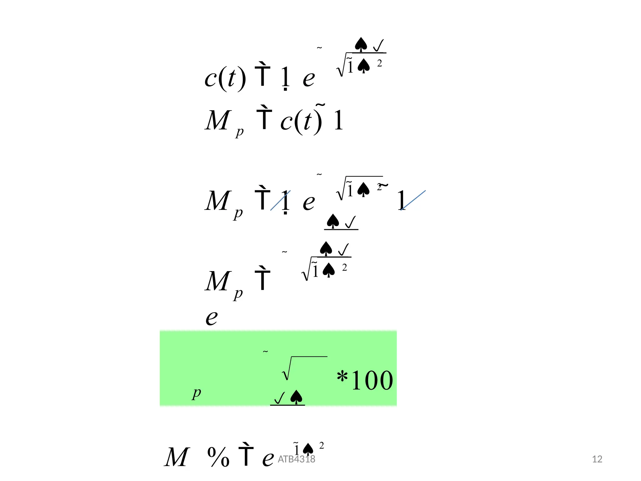
4. MAXIMUM OVERSHOOT(MP):
Maximum overshoot occur at peak time, t=tp
in above equation
n
en
t
2
1 t
1
2
c(t) 1 sin
1
2
n
p
t
Put,
1
2
c(t) 1
e
2
1 2
sin 1
. n
n
n
n
1
2
ATB4318 10
1 2
1 2
12
1
M 1 e
M p c(t) 1
c(t) 1 e
M
e
p
p
*100
ATB4318 12
M % e 1 2
p
52.
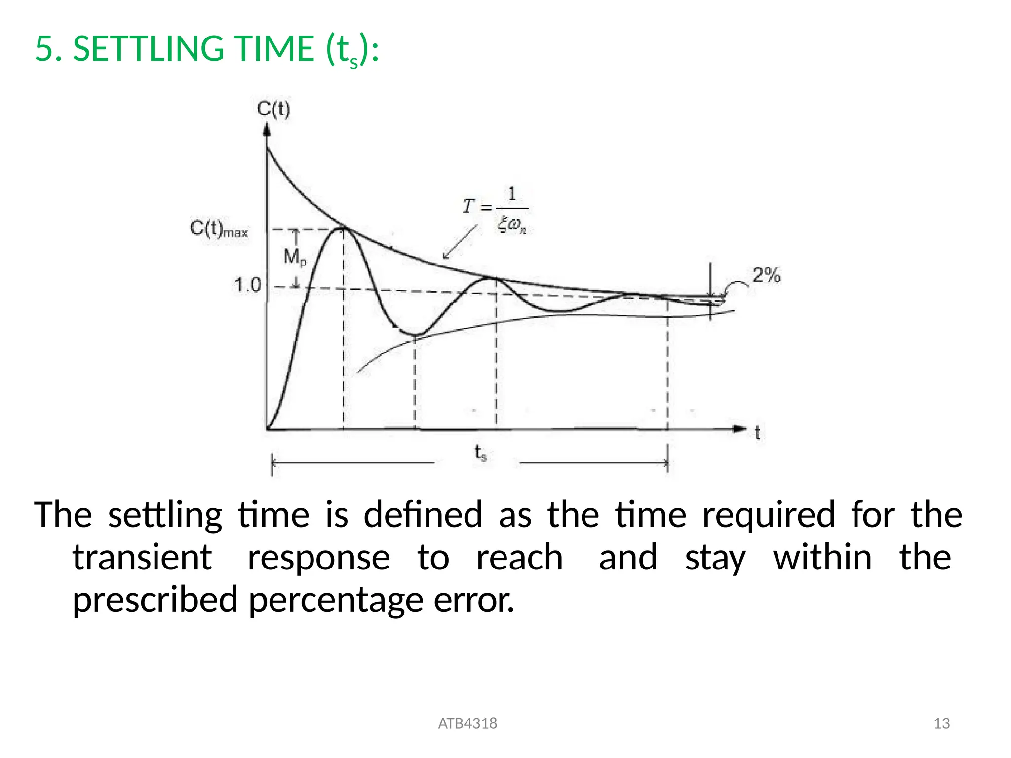
5. SETTLING TIME(ts):
The settling time is defined as the time required for the
transient response to reach and stay within the
prescribed percentage error.
ATB4318 13
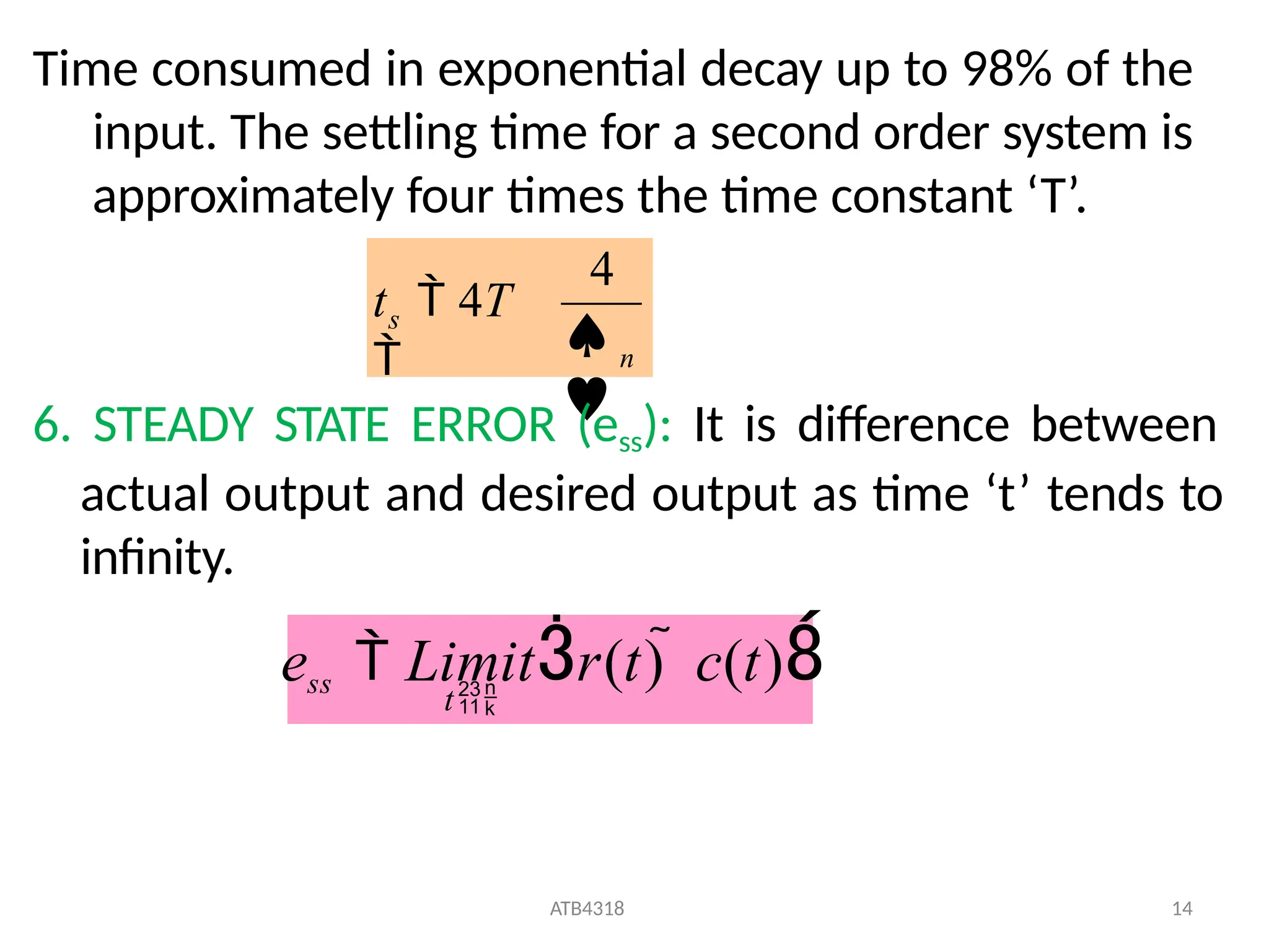
53.
Time consumed inexponential decay up to 98% of the
input. The settling time for a second order system is
approximately four times the time constant ‘T’.
n
s
4
t 4T
6. STEADY STATE ERROR (ess): It is difference between
actual output and desired output as time ‘t’ tends to
infinity.
ess Limitr(t) c(t)
ATB4318 14
t
54.
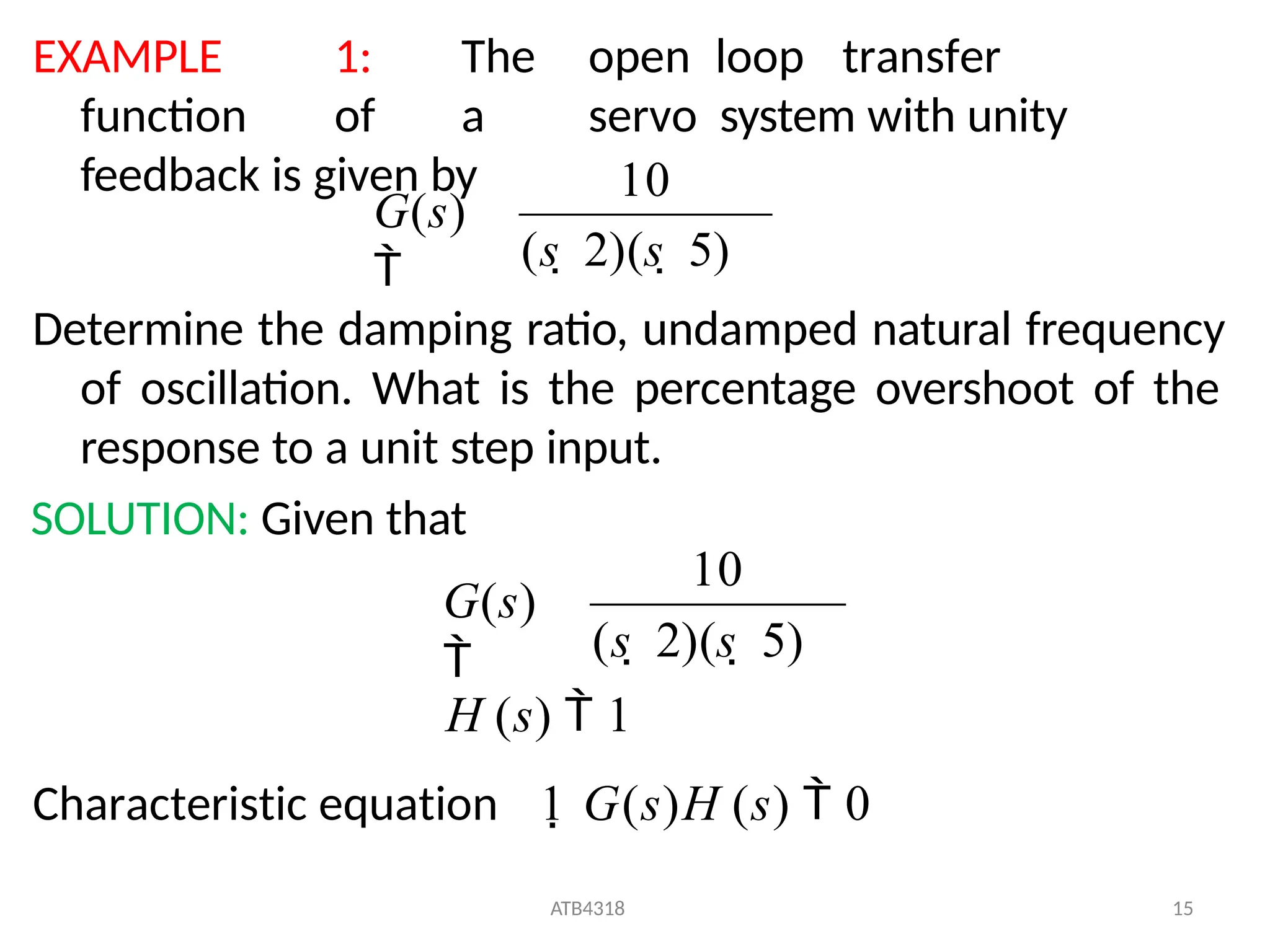
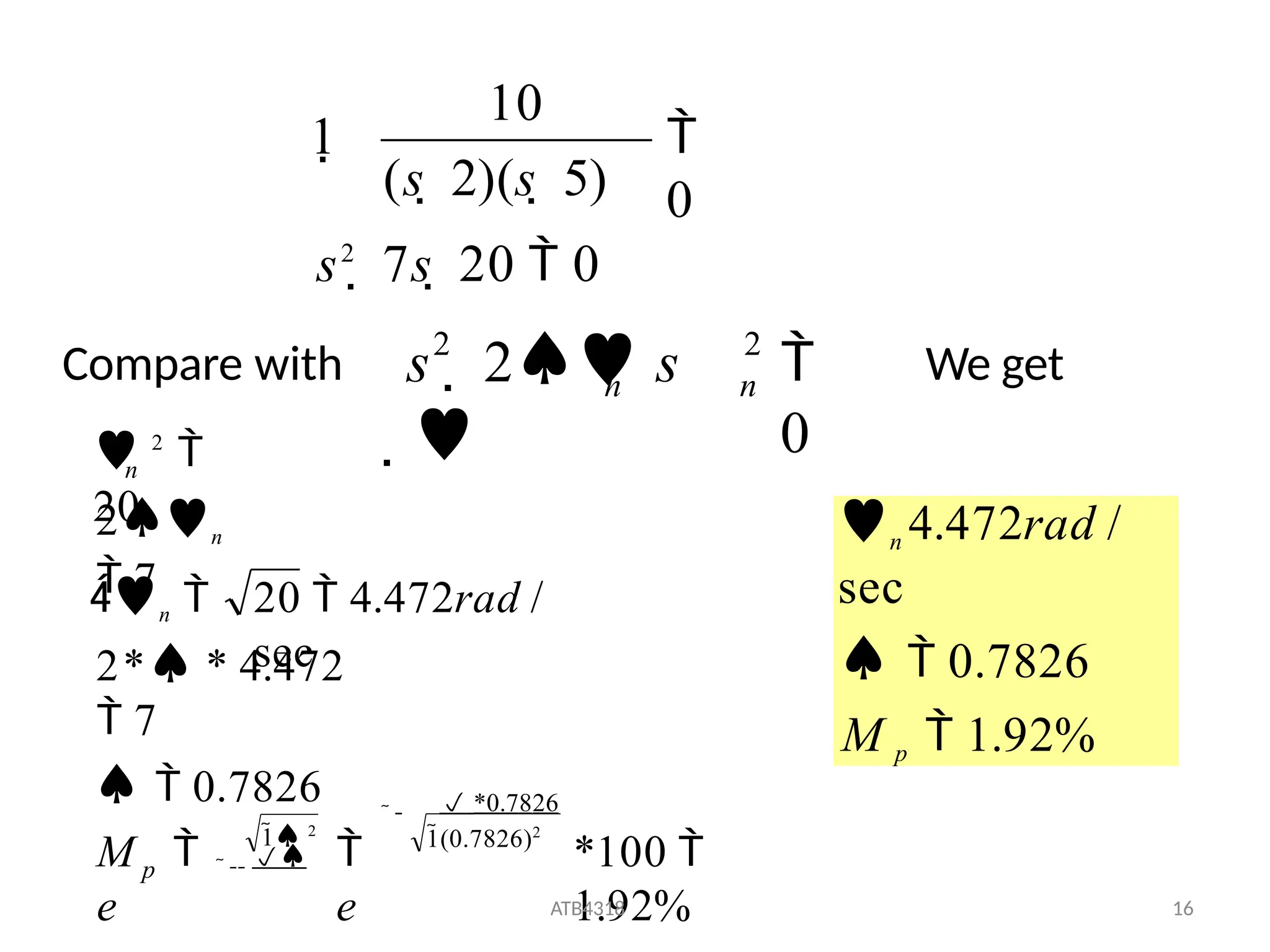
EXAMPLE 1: Theopen loop transfer
function of a servo system with unity
feedback is given by
Determine the damping ratio, undamped natural frequency
of oscillation. What is the percentage overshoot of the
response to a unit step input.
SOLUTION: Given that
(s 2)(s 5)
10
G(s)
(s 2)(s 5)
ATB4318 15
H (s) 1
Characteristic equation 1 G(s)H (s) 0
10
G(s)
55.
s2
7s 20 0
0
(s 2)(s 5)
10
1
Compare with
0
2
2
n
n
s 2 s
We get
*100
1.92%
ATB4318 16
2* * 4.472
7
0.7826
20 4.472rad /
sec
2
20
n
2n
7
1(0.7826)2
1 2
*0.7826
e
M
e
n
p
n 4.472rad /
sec
0.7826
M p 1.92%
56.
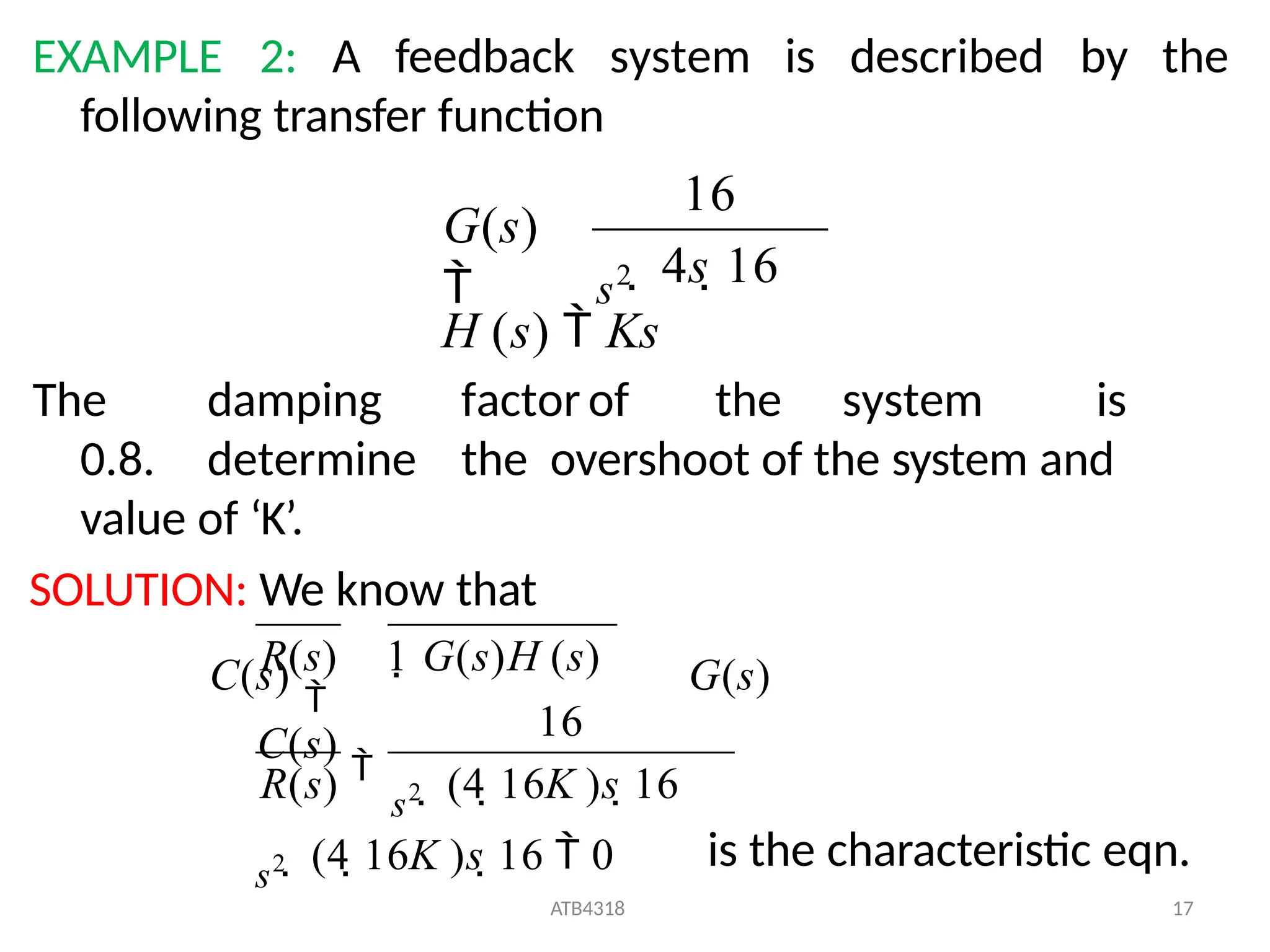
EXAMPLE 2: Afeedback system is described by the
following transfer function
4s 16
s2
G(s)
16
(4 16K )s 16 0
ATB4318 17
(4 16K )s 16
s2
R(s) s2
1 G(s)H (s)
16
R(s)
C(s)
H (s) Ks
The damping factor of the system is
0.8. determine the overshoot of the system and
value of ‘K’.
SOLUTION: We know that
C(s)
G(s)
is the characteristic eqn.
57.
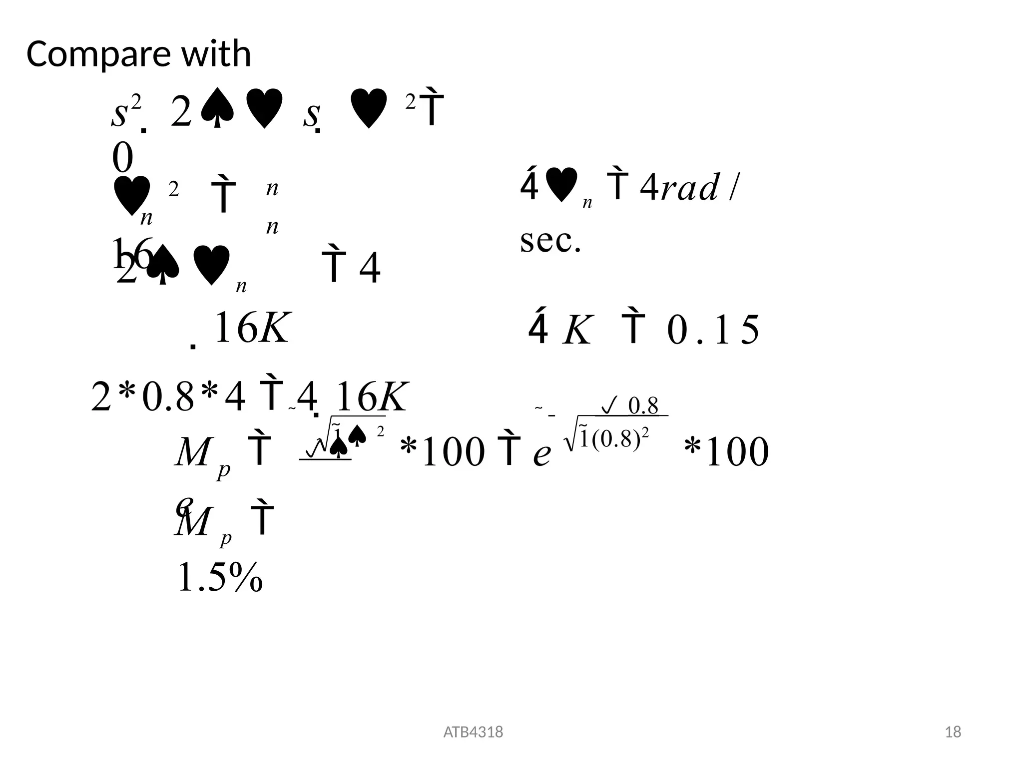
Compare with
s2
2s 2
0
n
n
2
16
n
2n 4
16K
2*0.8*4 4 16K
n 4rad /
sec.
K 0.15
p
M p
1.5%
ATB4318 18
1(0.8)2
*100 e *100
0.8
M
e
1 2
58.
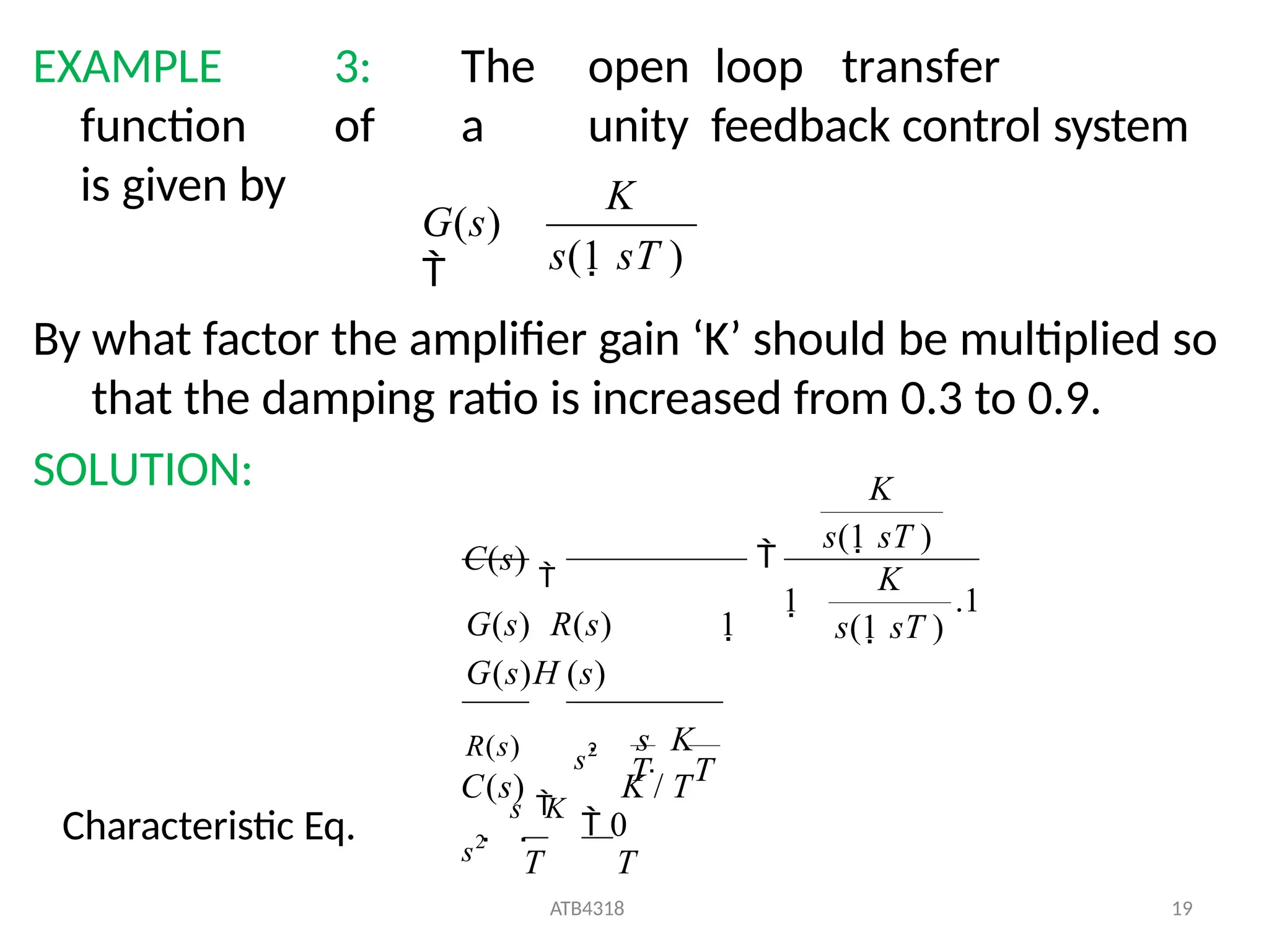
EXAMPLE 3: Theopen loop transfer
function of a unity feedback control system
is given by
By what factor the amplifier gain ‘K’ should be multiplied so
that the damping ratio is increased from 0.3 to 0.9.
SOLUTION:
s(1 sT )
G(s)
K
s
K
0
T T
ATB4318 19
.1
K
s(1 sT )
1
s(1 sT )
s2
s
K
R(s) s2
C(s)
G(s) R(s) 1
G(s)H (s)
C(s)
K / T
T T
K
Characteristic Eq.
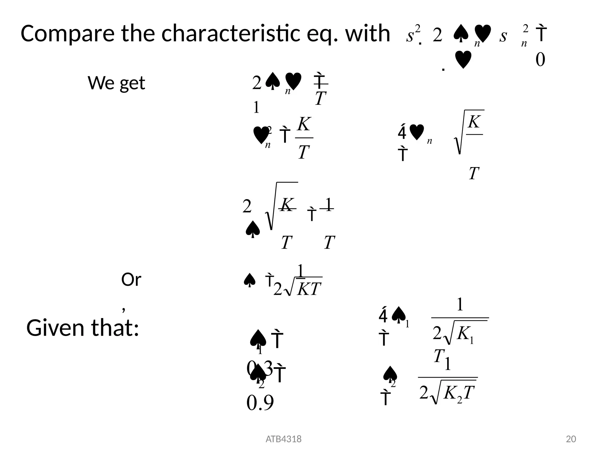
59.
Given that:
0
2
2
n
n
Compare thecharacteristic eq. with s 2 s
T
K
T
n
n
2
1
2
We get
K
1
T T
2
K
T
n
2 KT
1
Or
,
2
0.9
1
0.3
2
ATB4318 20
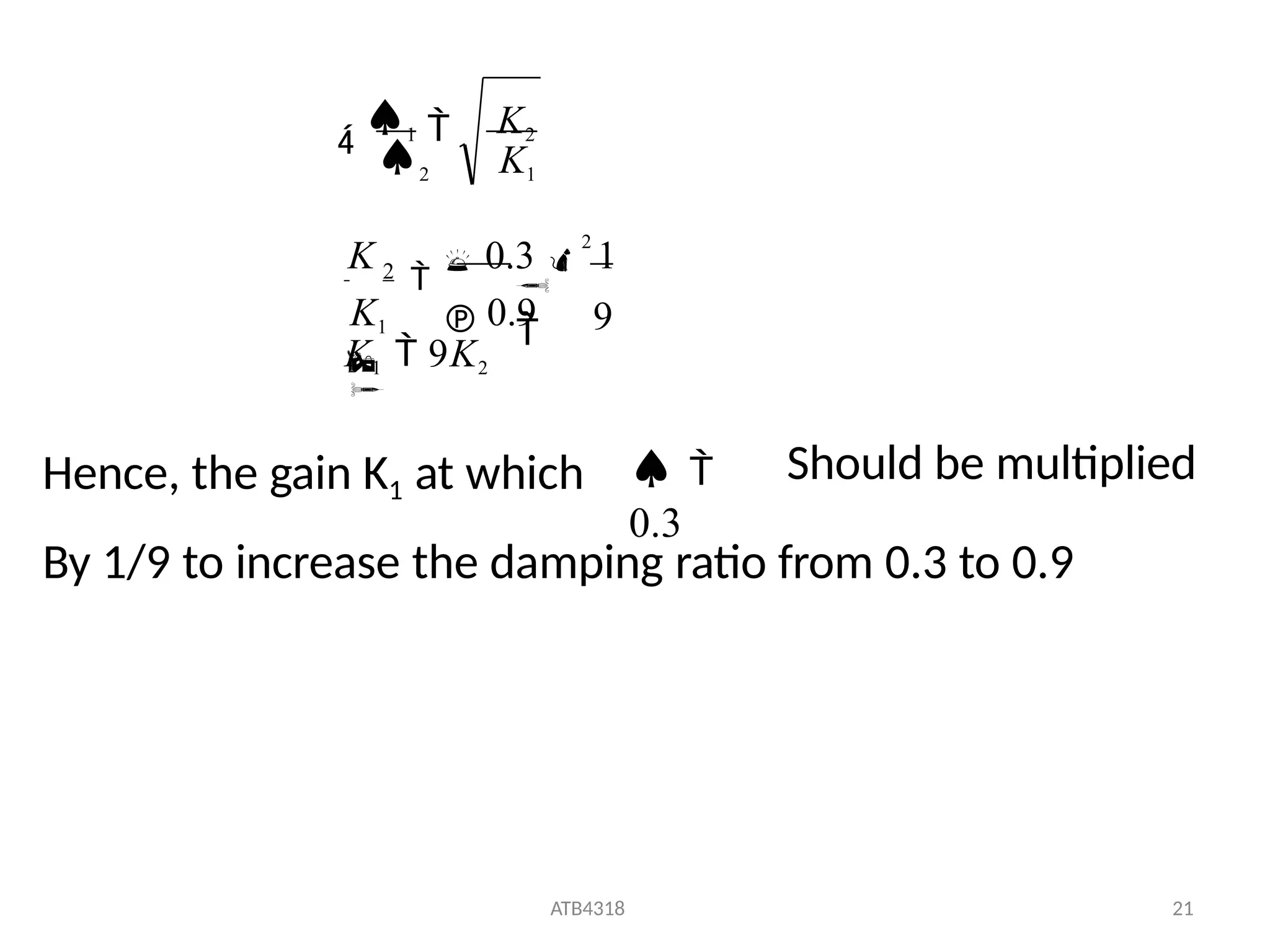
2 K T
2
1
2 K
T
1
1
1
60.
K1 9K2
ATB431821
K1 0.9
K 0.3
2
1
9
2
2 K1
1 K2
Hence, the gain K1 at which
0.3
Should be multiplied
By 1/9 to increase the damping ratio from 0.3 to 0.9
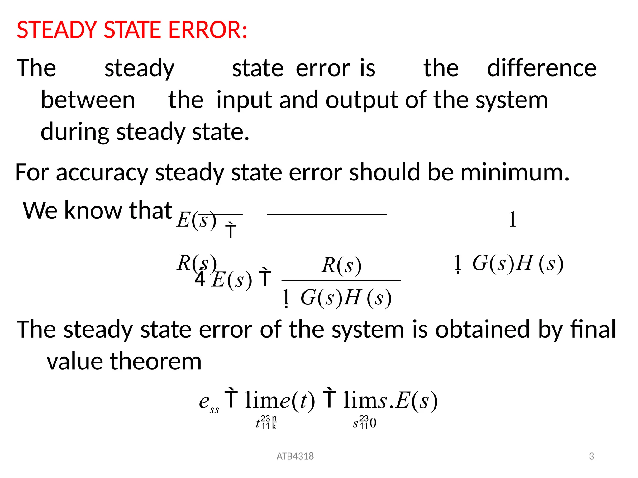
STEADY STATE ERROR:
Thesteady state error of the system is obtained by final
value theorem
ess lime(t) lims.E(s)
t s0
The steady state error is the difference
between the input and output of the system
during steady state.
For accuracy steady state error should be minimum.
We know thatE(s)
1
R(s) 1 G(s)H (s)
1 G(s)H (s)
ATB4318 3
R(s)
E(s)
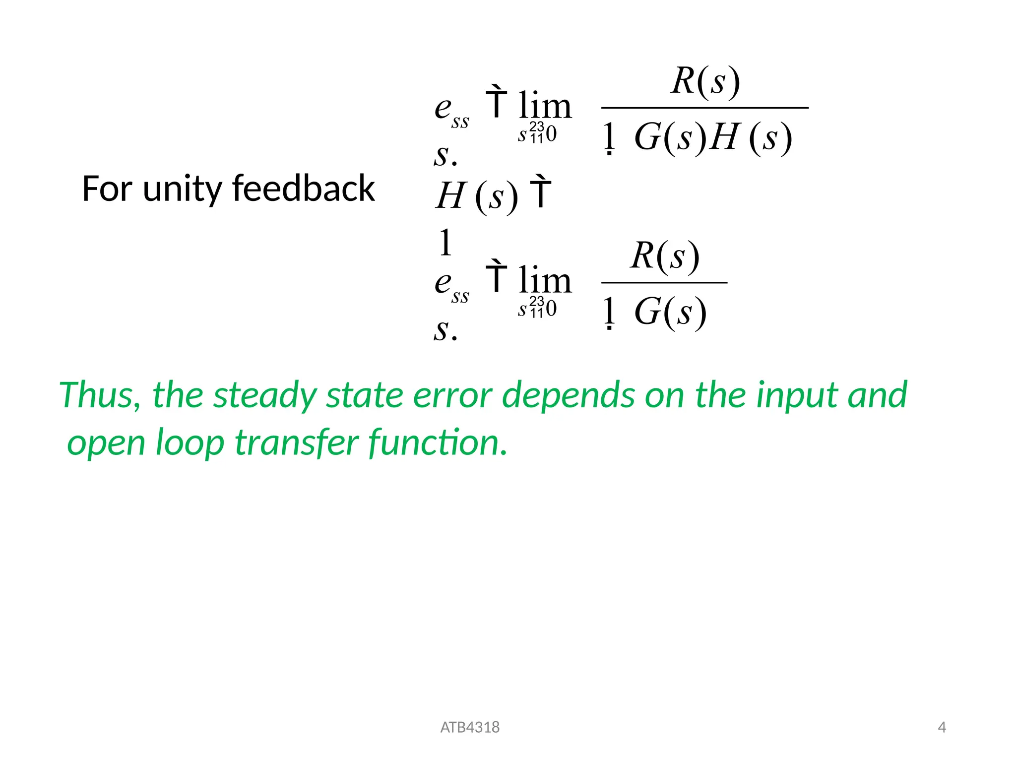
63.
R(s)
ATB4318 4
H (s)
1
R(s)
ss
1 G(s)
e lim
s.
s0
ss
1 G(s)H (s)
e lim
s.
s0
For unity feedback
Thus, the steady state error depends on the input and
open loop transfer function.
64.
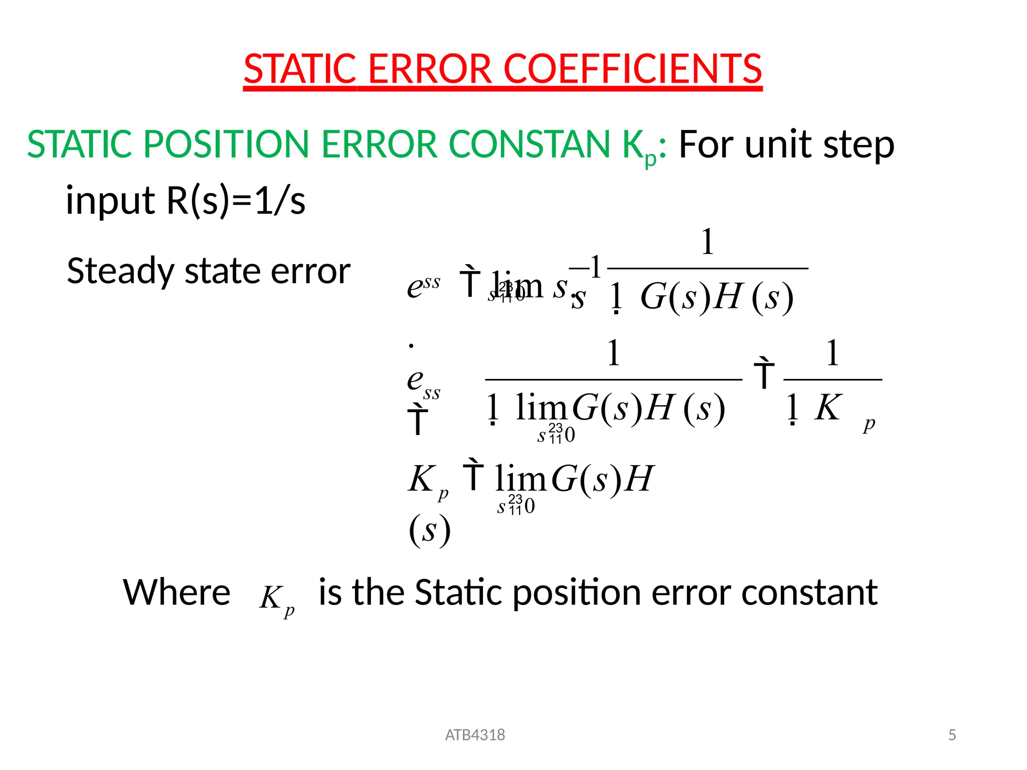
STATIC ERROR COEFFICIENTS
STATICPOSITION ERROR CONSTAN Kp: For unit step
input R(s)=1/s
1
ATB4318 5
1
1
s0
Kp limG(s)H
(s)
s0
p
ss
e
ss
s0 s 1 G(s)H (s)
e lim s.
1
.
1 limG(s)H (s) 1 K
Where Kp
is the Static position error constant
Steady state error
65.
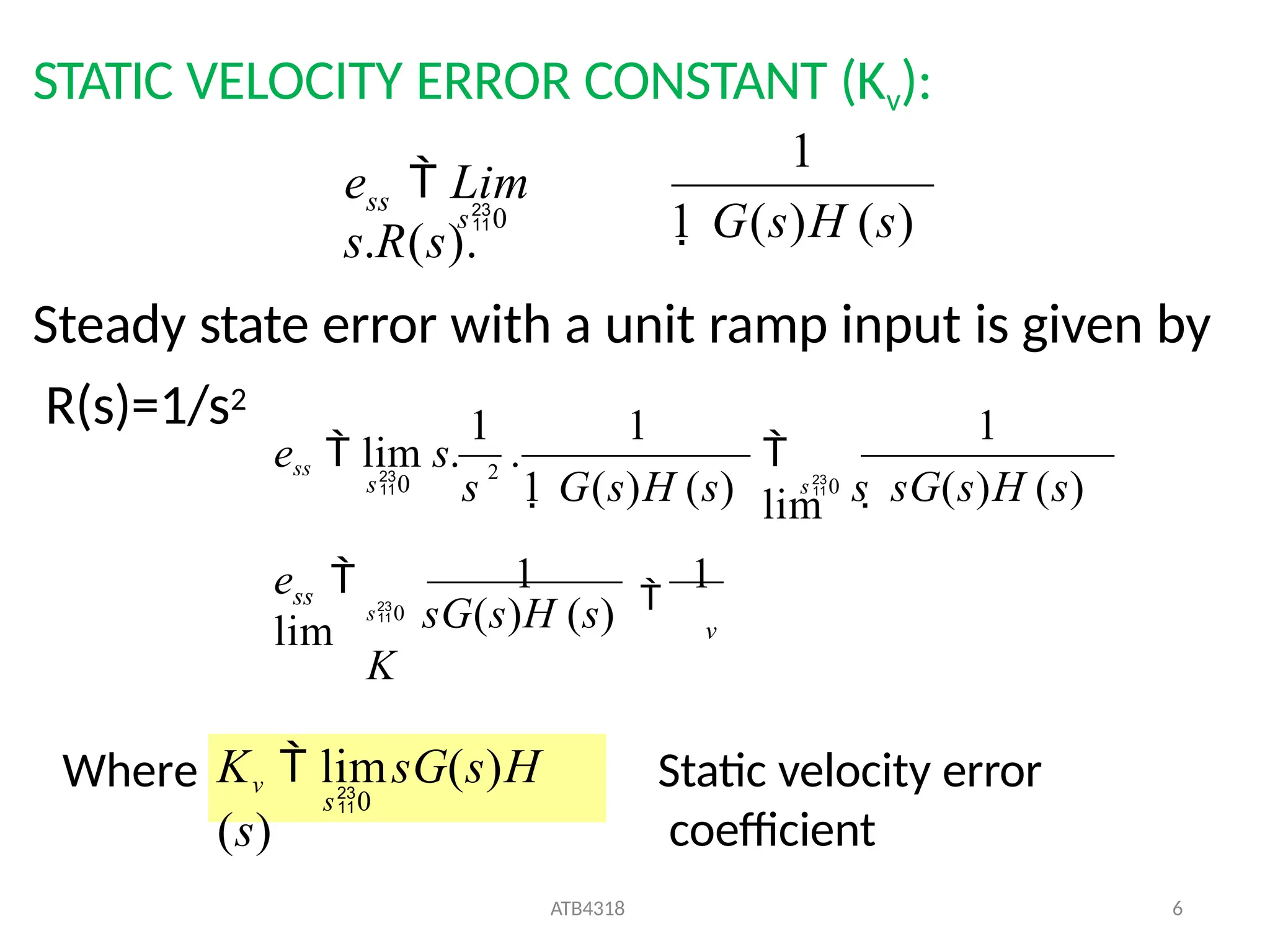
STATIC VELOCITY ERRORCONSTANT (Kv):
Steady state error with a unit ramp input is given by
R(s)=1/s2
1
ss
1 G(s)H (s)
e Lim
s.R(s).
s0
v
ss
e
lim
s0 sG(s)H (s)
K
1
1
1
1 1
lim
s 1 G(s)H (s)
ess lim s. 2
.
s0 s sG(s)H (s)
s0
Where s0
ATB4318 6
Kv limsG(s)H
(s)
Static velocity error
coefficient
66.
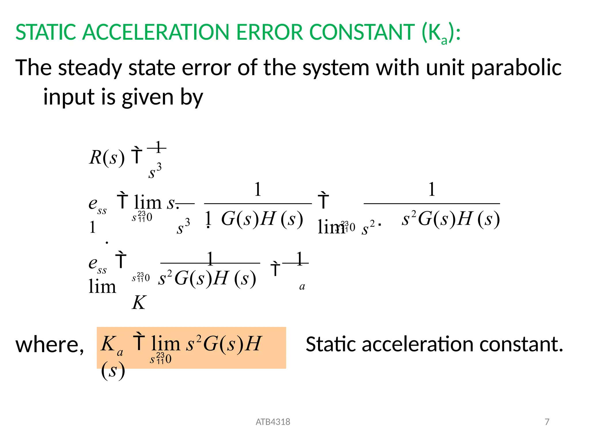
STATIC ACCELERATION ERRORCONSTANT (Ka):
The steady state error of the system with unit parabolic
input is given by
where,
a
ss
ss
e
lim
s0 s2
G(s)H (s)
K
s2
G(s)H (s)
s3
R(s)
1
1
lim
s0 s2
1
s3 1 G(s)H (s)
1
1
e lim s.
1
.
s0
a
ATB4318 7
s0
K lim s2
G(s)H
(s)
Static acceleration constant.
67.
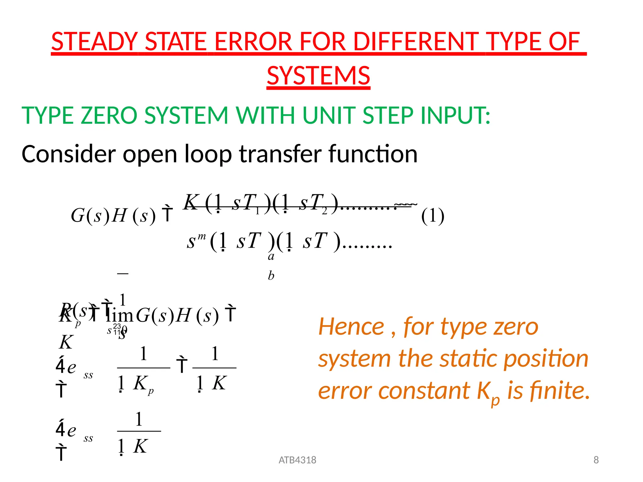
STEADY STATE ERRORFOR DIFFERENT TYPE OF
SYSTEMS
1 K
ATB4318 8
Kp limG(s)H (s)
K
TYPE ZERO SYSTEM WITH UNIT STEP INPUT:
Consider open loop transfer function
G(s)H (s)
K (1 sT1 )(1 sT2 )..........
(1)
sm
(1 sT )(1 sT ).........
a
b
R(s)
1
s
ss
ss
e
s0
e
1 Kp 1 K
1
1 1
Hence , for type zero
system the static position
p
error constant K is finite.
68.
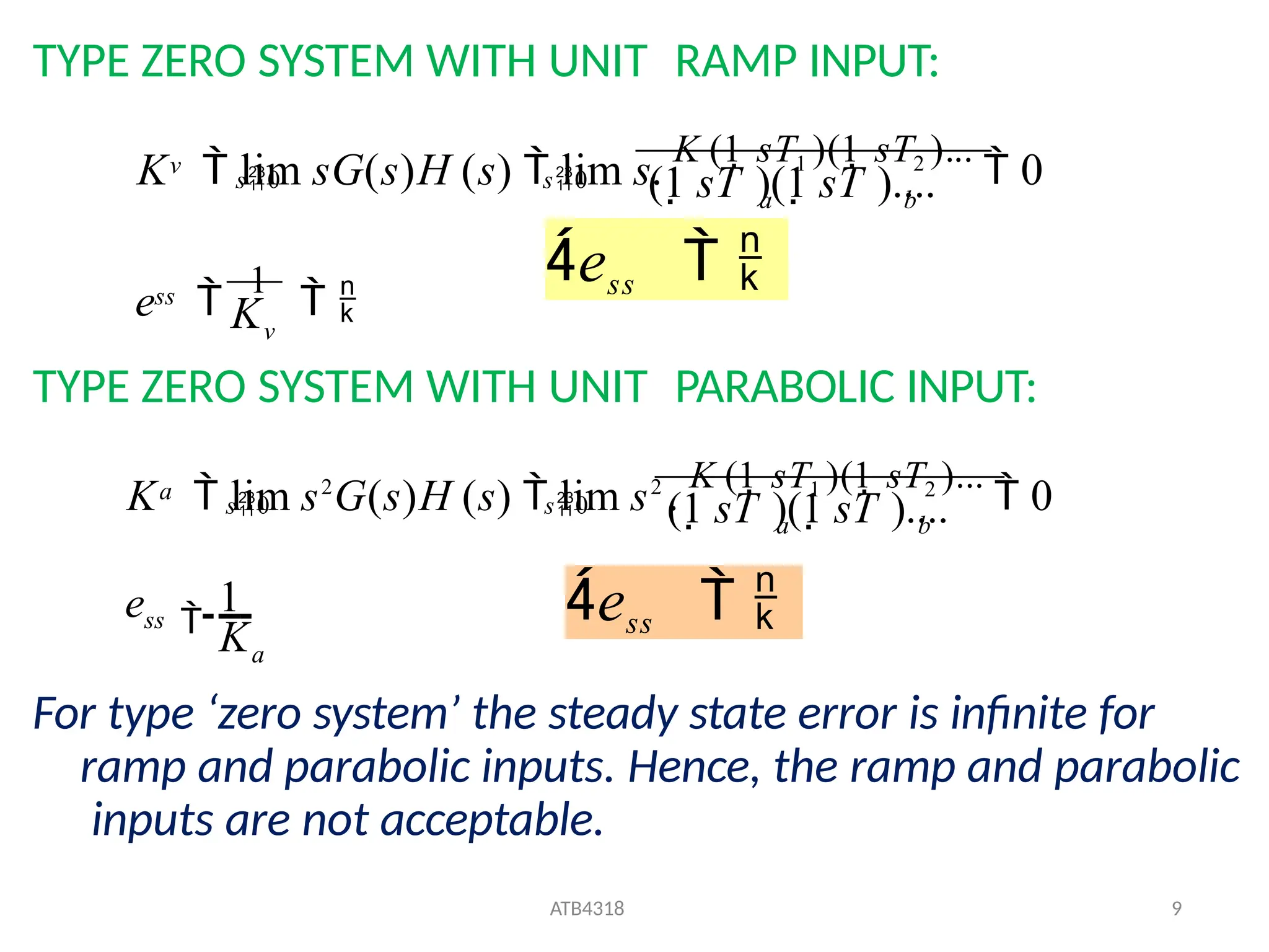
TYPE ZERO SYSTEMWITH UNIT RAMP INPUT:
TYPE ZERO SYSTEM WITH UNIT PARABOLIC INPUT:
For type ‘zero system’ the steady state error is infinite for
ramp and parabolic inputs. Hence, the ramp and parabolic
inputs are not acceptable.
v
ss
b
a
v
(1 sT )(1 sT )....
K lim sG(s)H (s) lim s.
K (1 sT1 )(1 sT2 )...
0
s0 s0
K
e
1
ess
a
ATB4318 9
ss
b
a
a
K
e
(1 sT )(1 sT )....
K lim s2
G(s)H (s) lim s2
.
K (1 sT1 )(1 sT2 )...
0
s0 s0
1 ess
69.
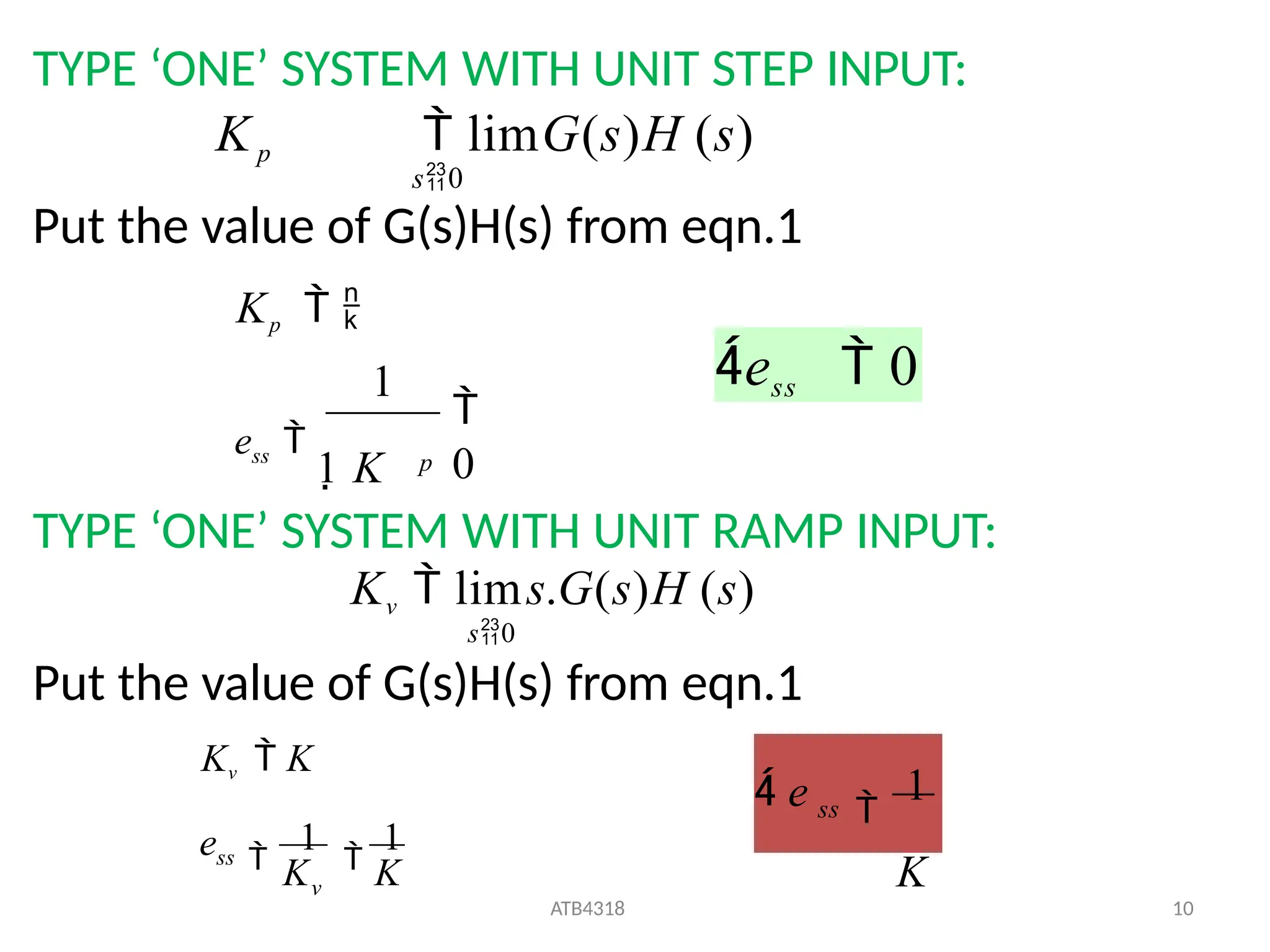
TYPE ‘ONE’ SYSTEMWITH UNIT STEP INPUT:
Kp limG(s)H (s)
s0
Put the value of G(s)H(s) from eqn.1
Kp
TYPE ‘ONE’ SYSTEM WITH UNIT RAMP INPUT:
Kv lims.G(s)H (s)
s0
Put the value of G(s)H(s) from eqn.1
0
1
p
ess
1 K
ess 0
K K
e
Kv K
v
ss
1
1
ss
ATB4318 10
1
K
e
70.
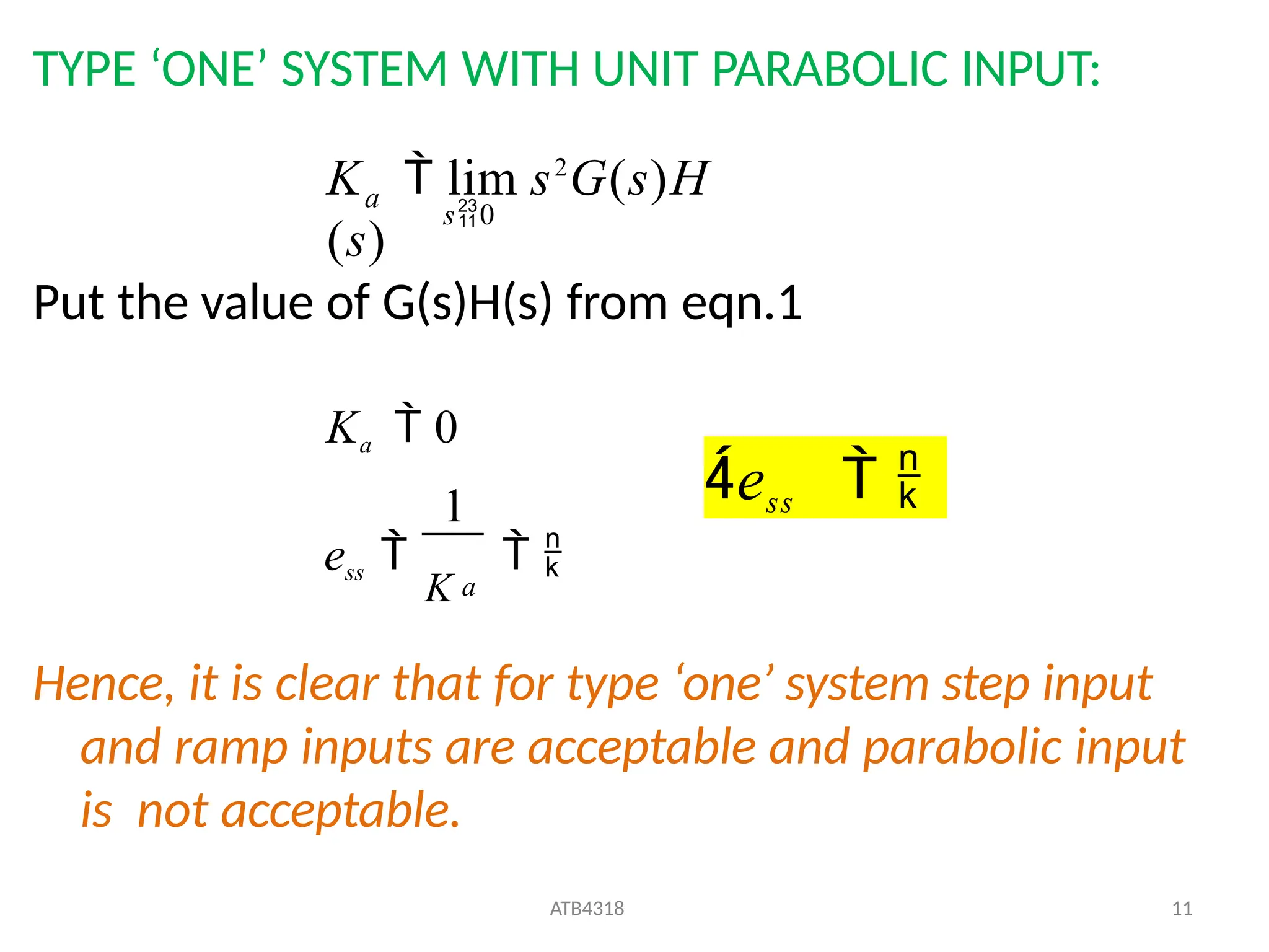
TYPE ‘ONE’ SYSTEMWITH UNIT PARABOLIC INPUT:
Put the value of G(s)H(s) from eqn.1
Hence, it is clear that for type ‘one’ system step input
and ramp inputs are acceptable and parabolic input
is not acceptable.
a
s0
K lim s2
G(s)H
(s)
ess
K
ATB4318 11
Ka 0
1
a
ess
71.
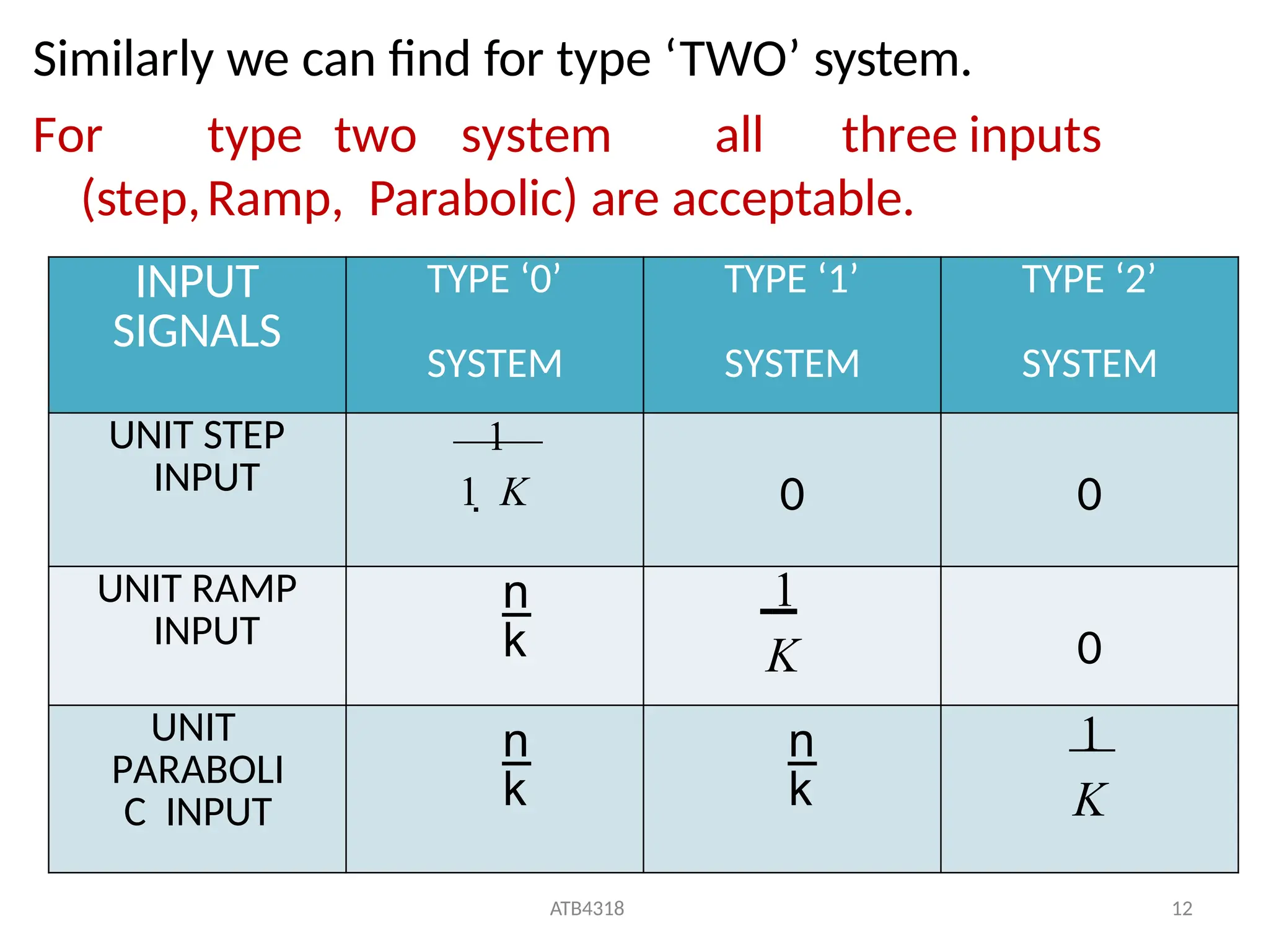
Similarly we canfind for type ‘TWO’ system.
For type two system all three inputs
(step,Ramp, Parabolic) are acceptable.
INPUT
SIGNALS
TYPE ‘0’
SYSTEM
TYPE ‘1’
SYSTEM
TYPE ‘2’
SYSTEM
UNIT STEP
INPUT
1
1 K 0 0
UNIT RAMP
INPUT 1
K 0
UNIT
PARABOLI
C INPUT
1
K
ATB4318 12
72.
DYNAMIC ERROR COEFFICIENT:
Forthe steady-state error, the static error coefficients
gives the limited information.
The error function is given by
The eqn.(2) can be expressed in polynomial form
(ascending power of ‘s’)
E(s)
1
R(s)
1 G(s)H (s)
For unity feedback system
(1)
(2)
ATB4318 13
E(s)
1
R(s) 1 G(s)
73.
1
s
1
s2
........ (3)
K2 K3
E(s)
1
R(s) K1
Or, E(s)
1
R(s)
1
sR(s)
1
s2
R(s)....... (4)
K1 K2 K3
Take inverse Laplace of eqn.(4), the error is given by
r (t) ....... (5)
1
K1 K2 K3
e(t)
1
r(t)
1
r(t)
s0
Steady state error is given by
ess
limsE(s)
Let
1
ATB4318 14
R(s)
s
74.
1
ATB4318 15
2
1
1 11
1 1
K
ess
ss
K1
1
.s. s .
.......
K2 s K3 s
e lim s. .
s
s0
Similarly, for other test signal we can find steady state
error.
K1 , K2 ,
K3 .......
are known as “Dynamic error
coefficients”
75.
EXAMPLE 1: Theopen loop transfer function of unity
feedback system is given by
Determine the static error coefficients K p , Kv , Ka
SOLUTION:
(1 0.1s)(s 10)
50
G(s)
0
ATB4318 16
(1 0.1s)(s 10)
50
lim
s2
Ka s G(s)H
(s) 2
0
(1 0.1s)(s 10)
50
lim
s.
5
50
lim
s0 (1 0.1s)(s 10)
s0
s0
s0
Kv lim s.G(s)H
(s)
s0
Kp limG(s)H (s)
76.
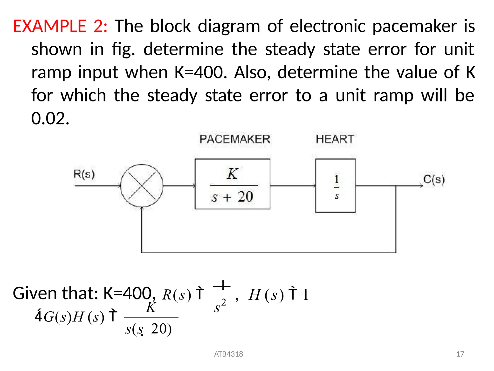
EXAMPLE 2: Theblock diagram of electronic pacemaker is
shown in fig. determine the steady state error for unit
ramp input when K=400. Also, determine the value of K
for which the steady state error to a unit ramp will be
0.02.
s2
Given that: K=400, R(s)
1
, H (s) 1
s(s 20)
ATB4318 17
G(s)H (s)
K
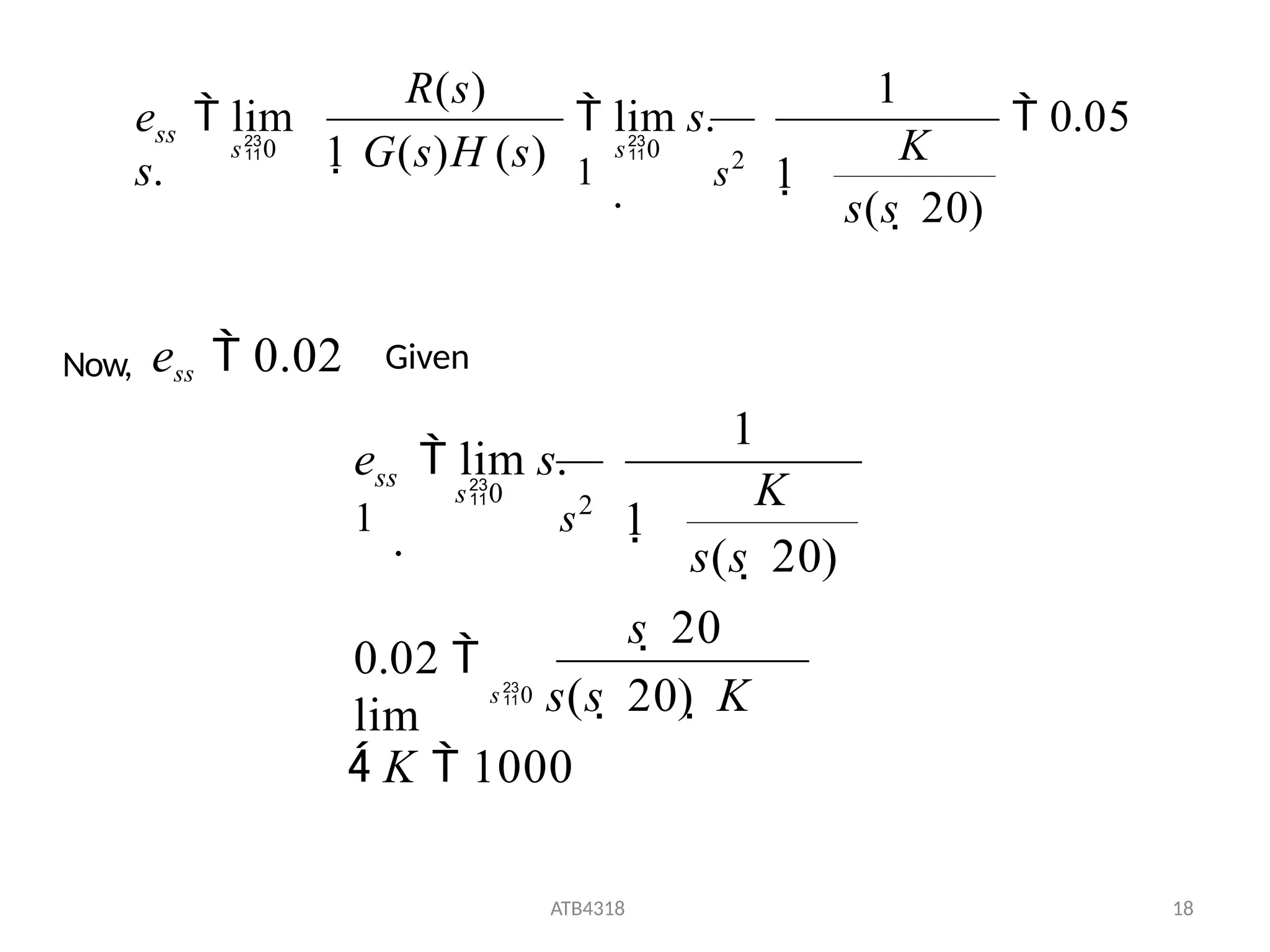
77.
0.05
1
1
K
s(s 20)
1 G(s)H (s)
R(s)
e lim
s. s2
lim s.
1
.
s0
s0
ss
Now, ess 0.02 Given
K 1000
ATB4318 18
s 20
0.02
lim
s0 s(s 20) K
s(s 20)
1
1
K
s2
e lim s.
1
.
s0
ss
ATB4318 3
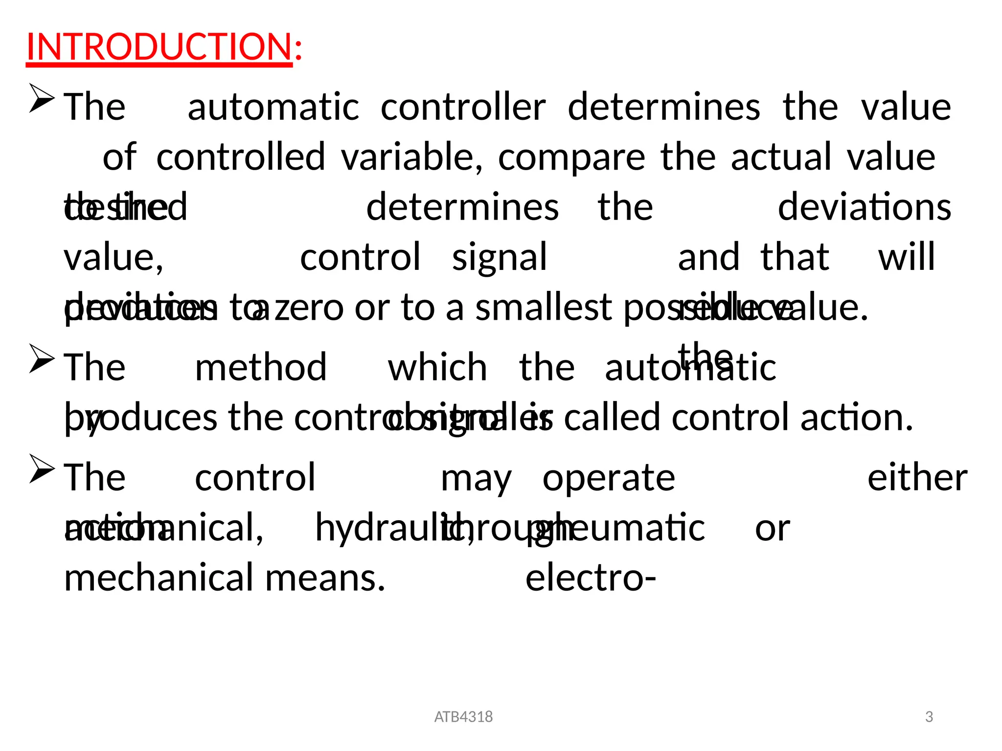
INTRODUCTION:
The automaticcontroller determines the value
of controlled variable, compare the actual value
to the determines
desired
value,
produces a
control signal
the deviations
and that will
reduce
the
deviation to zero or to a smallest possible value.
The method
by
which the automatic
controller
produces the control signal is called control action.
The control
action
may operate
through
either
mechanical, hydraulic, pneumatic or
electro-
mechanical means.
80.
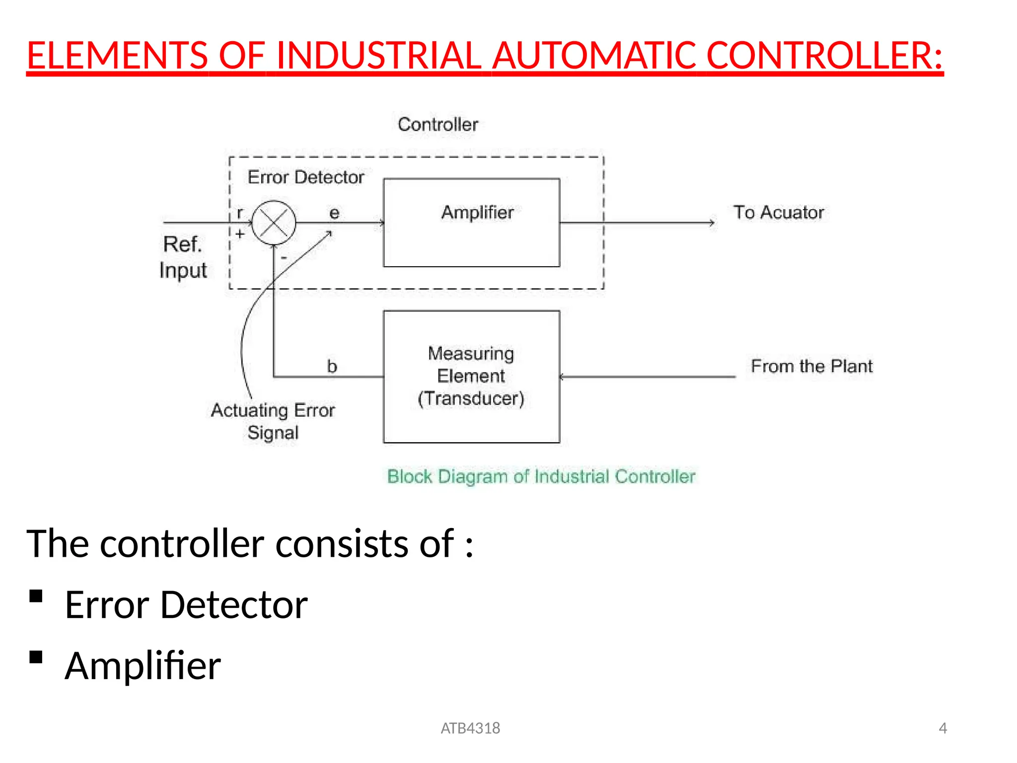
ELEMENTS OF INDUSTRIALAUTOMATIC CONTROLLER:
The controller consists of :
Error Detector
Amplifier
ATB4318 4
81.
ATB4318 5
Themeasuring element, which converts the
output variable to another suitable variable such
as displacement, pressure or electrical signals,
which can be used for comparing the output to
the reference input signal.
Deviation is the difference between controlled
variable and set point (reference input).
e=r-b
82.
ATB4318 6
CLASSIFICATION OFCONTROLLERS:
Controllers can be classified on the basis
of type of controlling action used. They
are classified as
i. Two position or ON-OFF controllers
ii. Proportional controllers
iii. Integral controllers
iv. Proportional-plus-integral controllers
v. Proportional-plus-derivative controllers
vi. Proportional-plus-integral-plus-
derivative controllers
83.
ATB4318 7
Controllers canalso be classified according to the power
source used for actuating mechanism, such as
electrical, electronics, pneumatic and hydraulic
controllers.
TWO POSITION CONTROL: This is also known as ON-OFF
or bang-bang control.
In this type ofcontrol the output of the controller is
quickly changed to either a maximum or minimum
value depending upon whether the controlled
variable (b) is greater or less than the set point.
Let m= output of the controller
M1=Maximum value of controller’s output
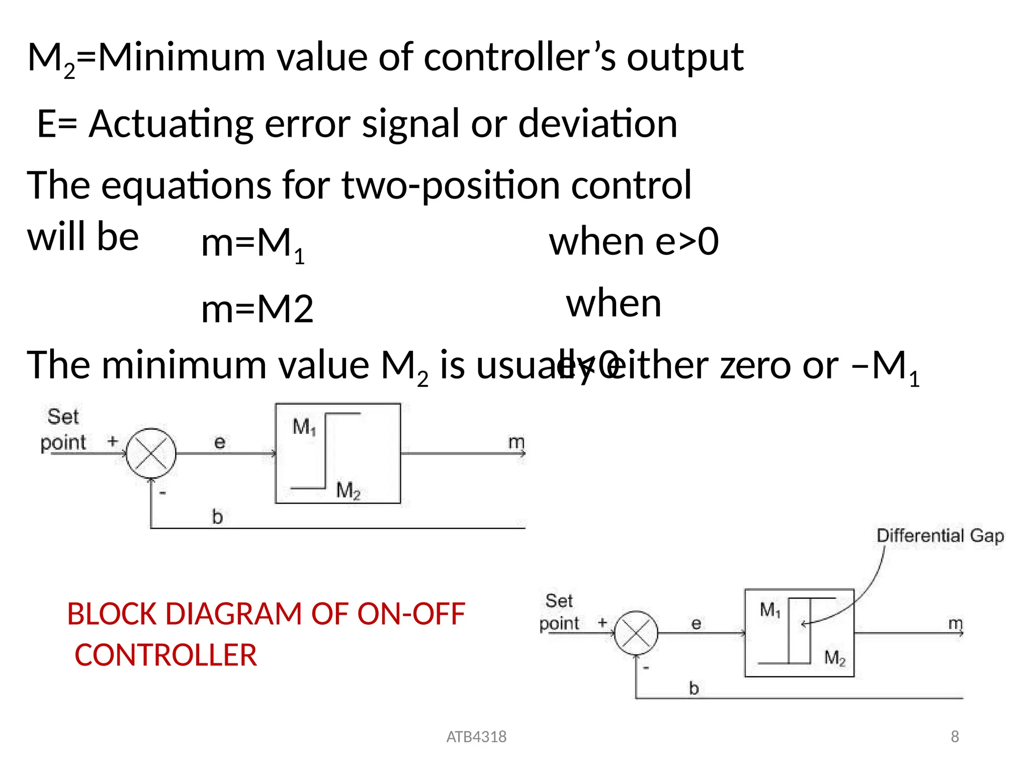
84.
M2=Minimum value ofcontroller’s output
E= Actuating error signal or deviation
The equations for two-position control
will be m=M1
m=M2
when e>0
when
e<0
The minimum value M2 is usually either zero or –M1
BLOCK DIAGRAM OF ON-OFF
CONTROLLER
ATB4318 8
85.
ATB4318 9
Block diagramof two position controller is shown in
previous slide. In such type of controller there is an
overlap as the error increases through zero or
decreases through zero. This overlap creates a span
of error. During this span of error, there is no change
in controller output. This span of error is known as
dead zone or dead band.
Two position control mode are used in room air
conditioners, heaters, liquid level control in large
volume tank.
86.
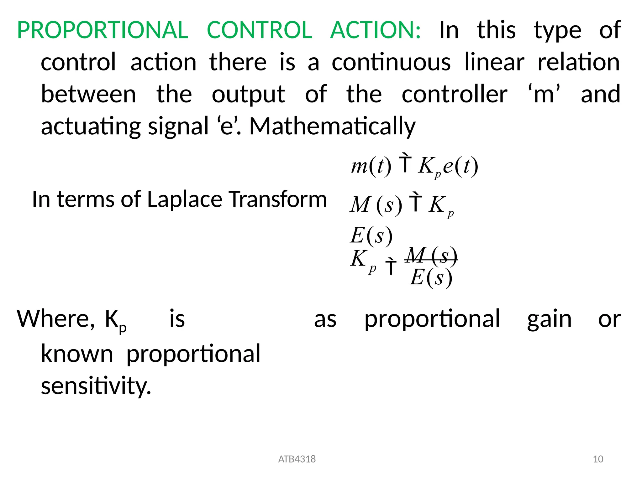
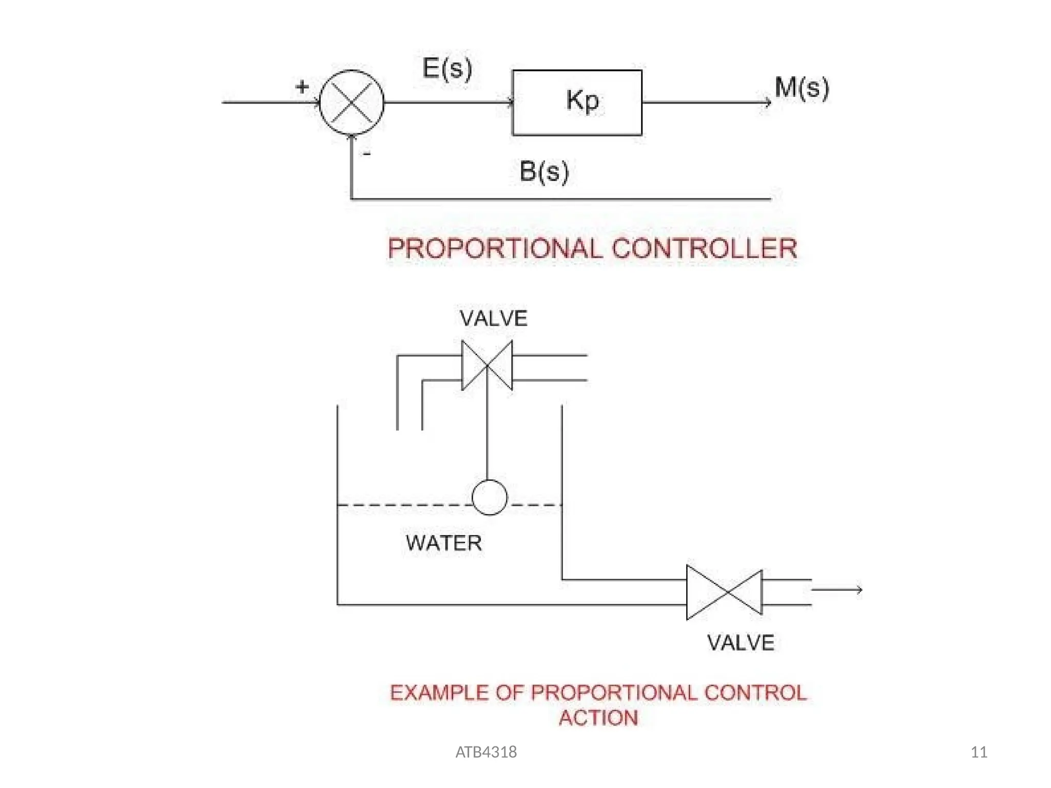
PROPORTIONAL CONTROL ACTION:In this type of
control action there is a continuous linear relation
between the output of the controller ‘m’ and
actuating signal ‘e’. Mathematically
m(t) Kpe(t)
Where, Kp is
known proportional
sensitivity.
as proportional gain or
E(s)
ATB4318 10
M (s)
M (s) Kp
E(s)
Kp
In terms of Laplace Transform
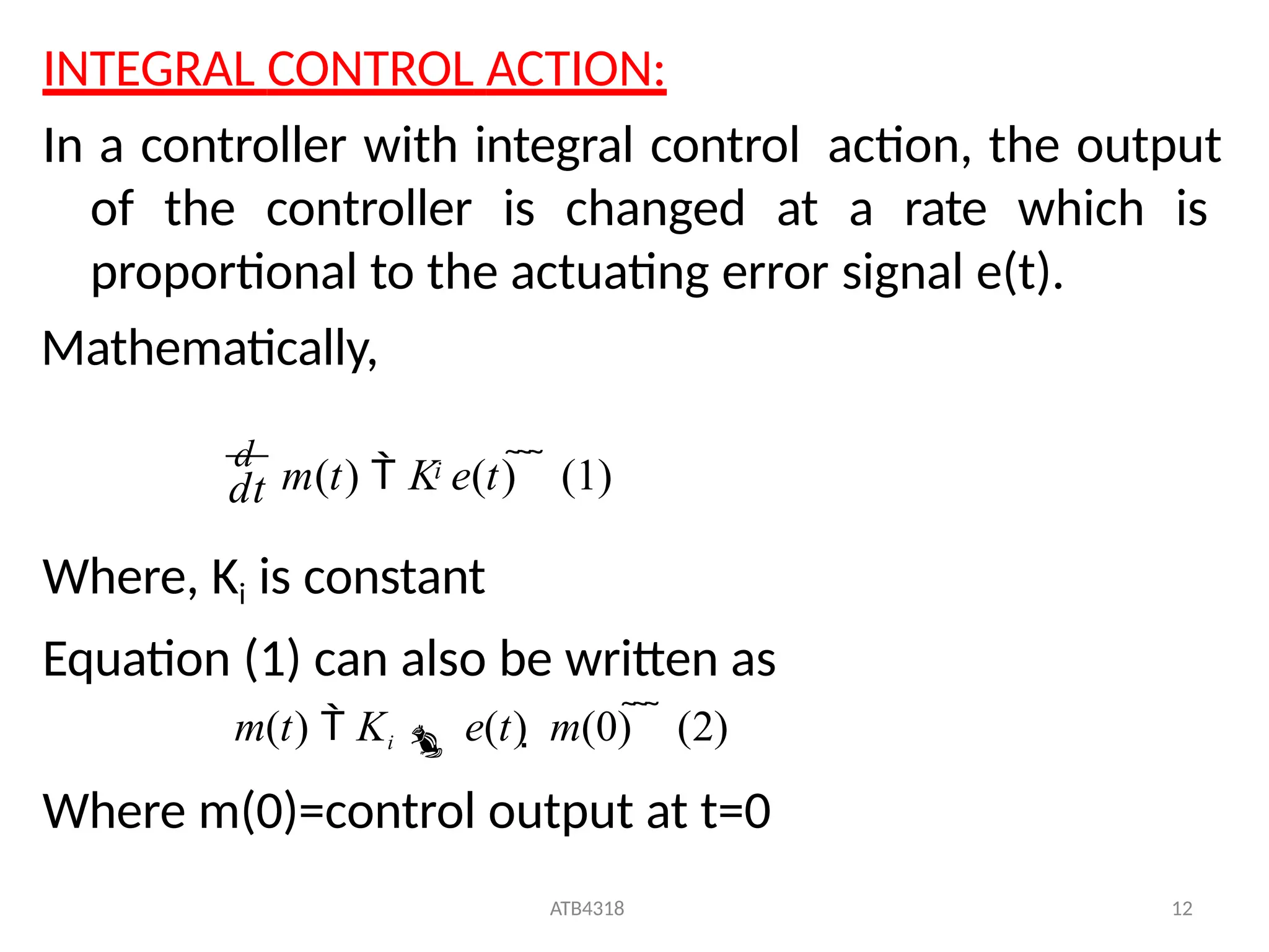
INTEGRAL CONTROL ACTION:
Ina controller with integral control action, the output
of the controller is changed at a rate which is
proportional to the actuating error signal e(t).
Mathematically,
Where, Ki is constant
Equation (1) can also be written as
m(t) Ki e(t) m(0) (2)
Where m(0)=control output at t=0
dt
ATB4318 12
d
m(t) K e(t) (1)
i
89.
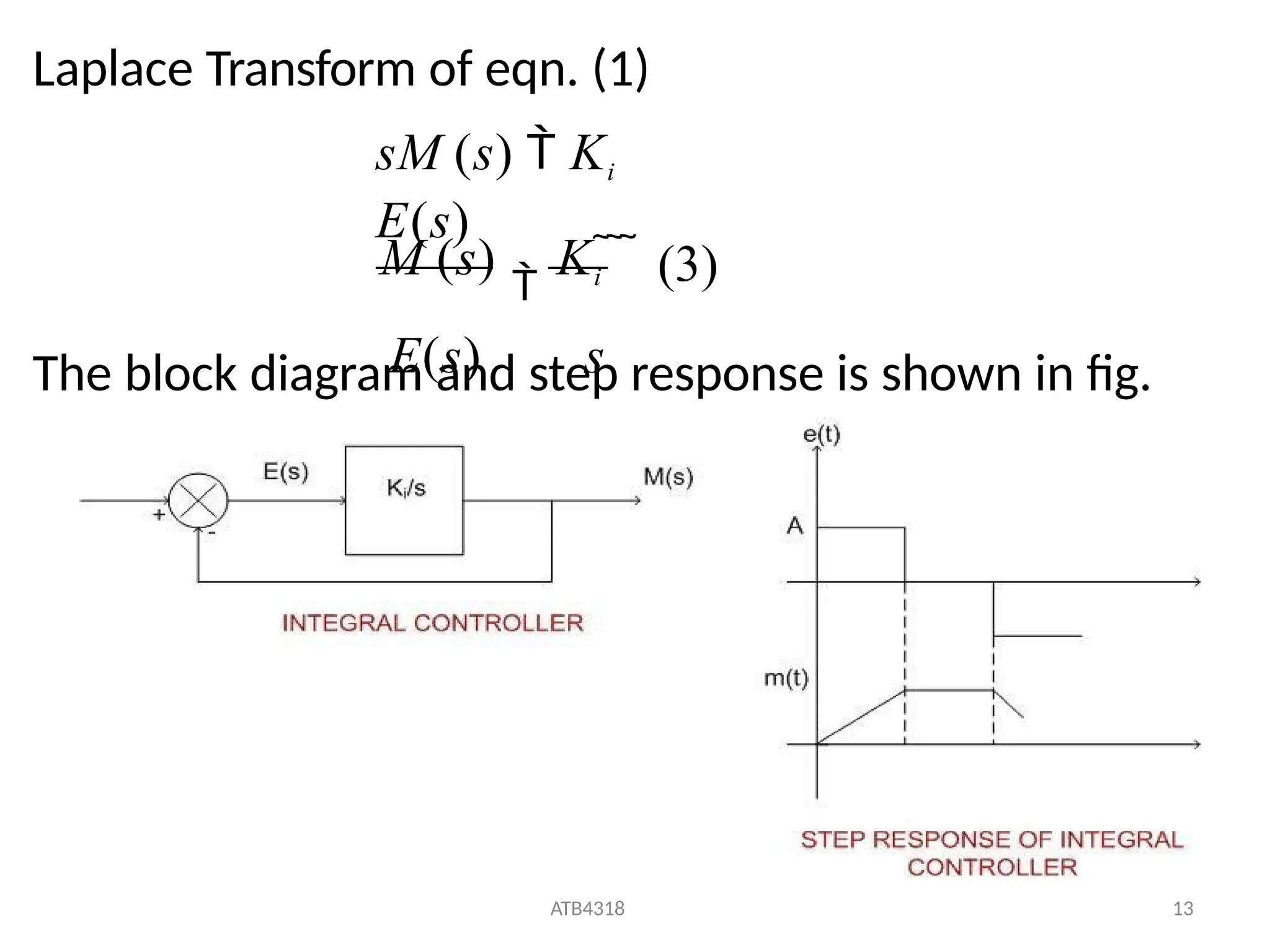
Laplace Transform ofeqn. (1)
The block diagram and step response is shown in fig.
(3)
M (s)
Ki
E(s) s
sM (s) Ki
E(s)
ATB4318 13
90.
ATB4318 14
The inverseof Ki is called integral time Ti and is defined
as time of change of output caused by a unit change
of actuating error signal. The step response is shown
in fig.
For positive error, the output of the controller is
ramp.
For zero error there is no change in the output of
the controller.
For negative error the output of the controller is
negative ramp.
91.
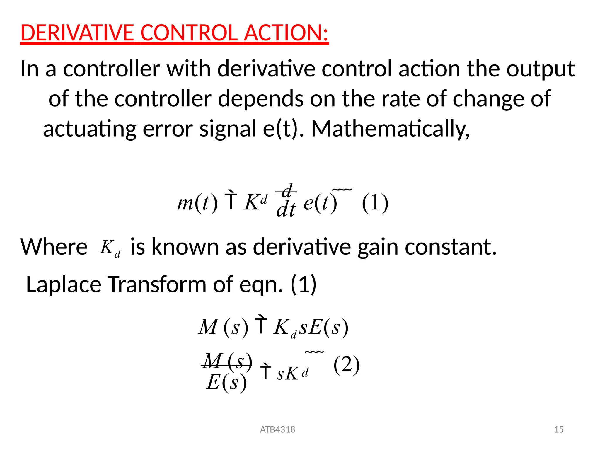
DERIVATIVE CONTROL ACTION:
Ina controller with derivative control action the output
of the controller depends on the rate of change of
actuating error signal e(t). Mathematically,
dt
m(t) K
d
e(t) (1)
d
Where Kd is known as derivative gain constant.
Laplace Transform of eqn. (1)
M (s) Kd sE(s)
(2)
ATB4318 15
E(s)
M (s)
sK d
92.
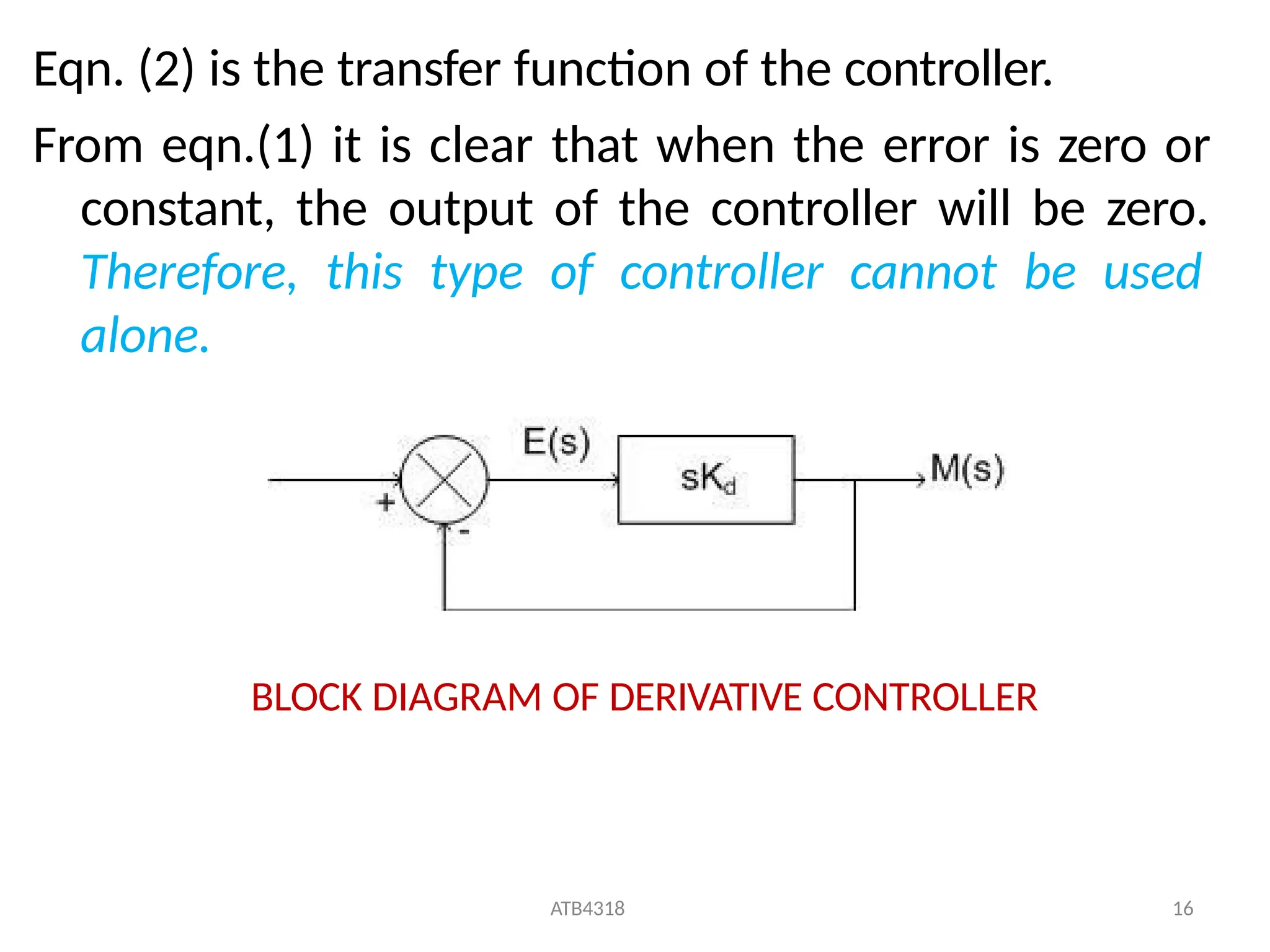
Eqn. (2) isthe transfer function of the controller.
From eqn.(1) it is clear that when the error is zero or
constant, the output of the controller will be zero.
Therefore, this type of controller cannot be used
alone.
BLOCK DIAGRAM OF DERIVATIVE CONTROLLER
ATB4318 16
93.
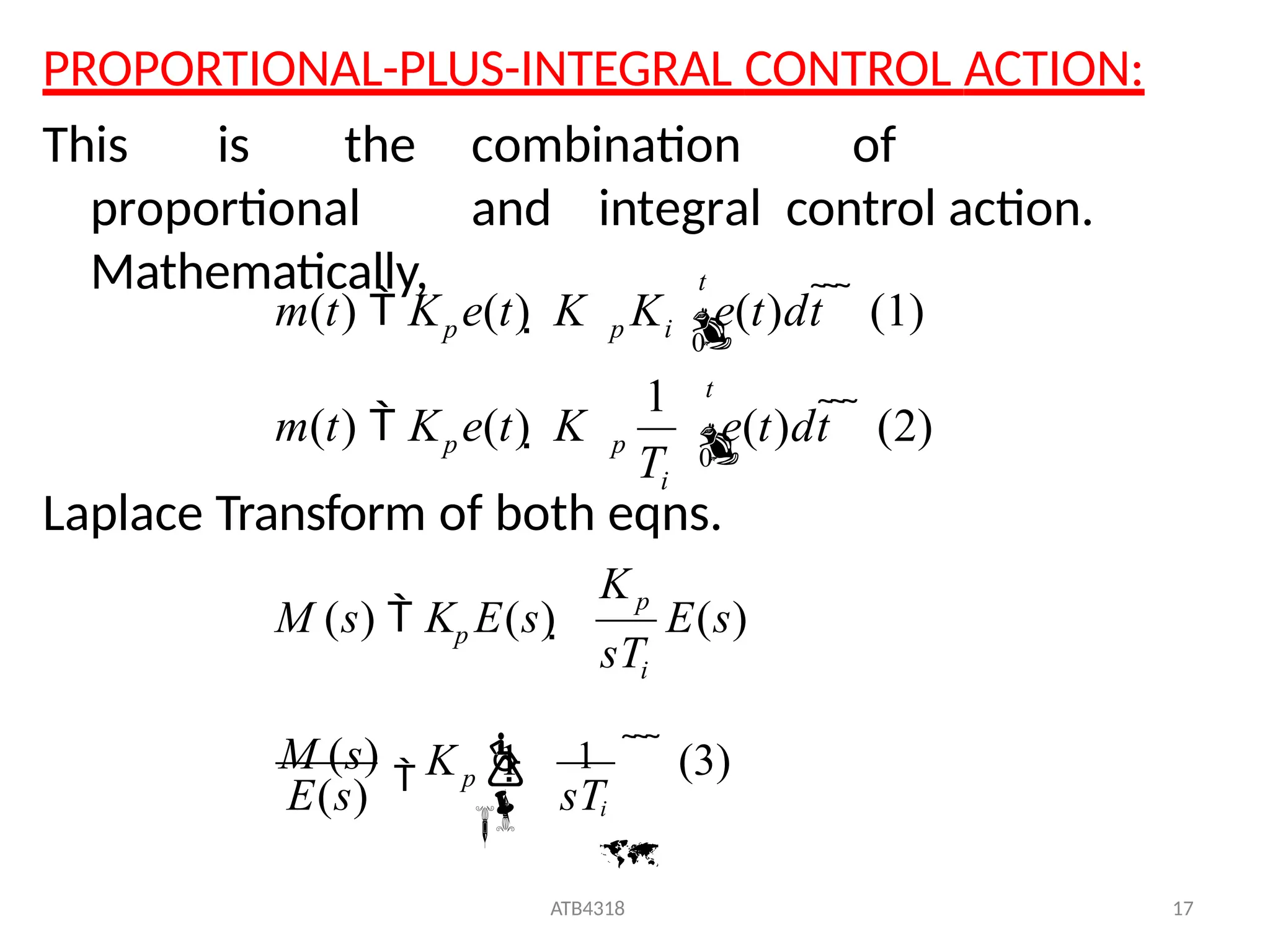
PROPORTIONAL-PLUS-INTEGRAL CONTROL ACTION:
Thisis the combination of
proportional and integral control action.
Mathematically,
Laplace Transform of both eqns.
p i
1
e(t)dt (1)
0
0
t
e(t)dt (2)
i
p p
m(t) K e(t) K
t
p
m(t) K e(t) K K
T
(3)
ATB4318 17
E(s)
M (s)
E(s)
1
i
p
i
p
p
M (s) K E(s)
sT
K 1
sT
K
94.
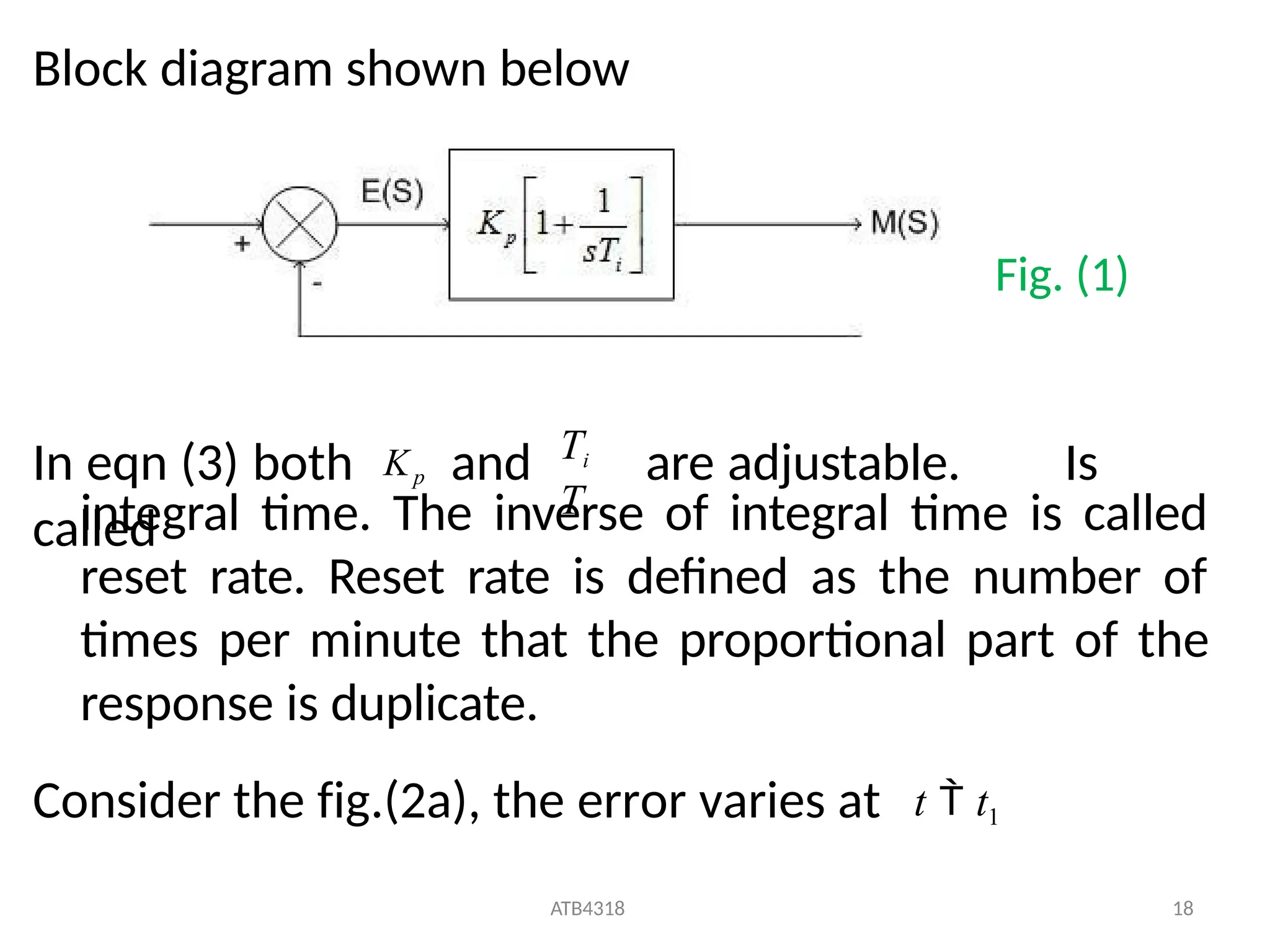
Block diagram shownbelow
In eqn (3) both Kp and are adjustable. Is
called
Ti
Ti
ATB4318 18
integral time. The inverse of integral time is called
reset rate. Reset rate is defined as the number of
times per minute that the proportional part of the
response is duplicate.
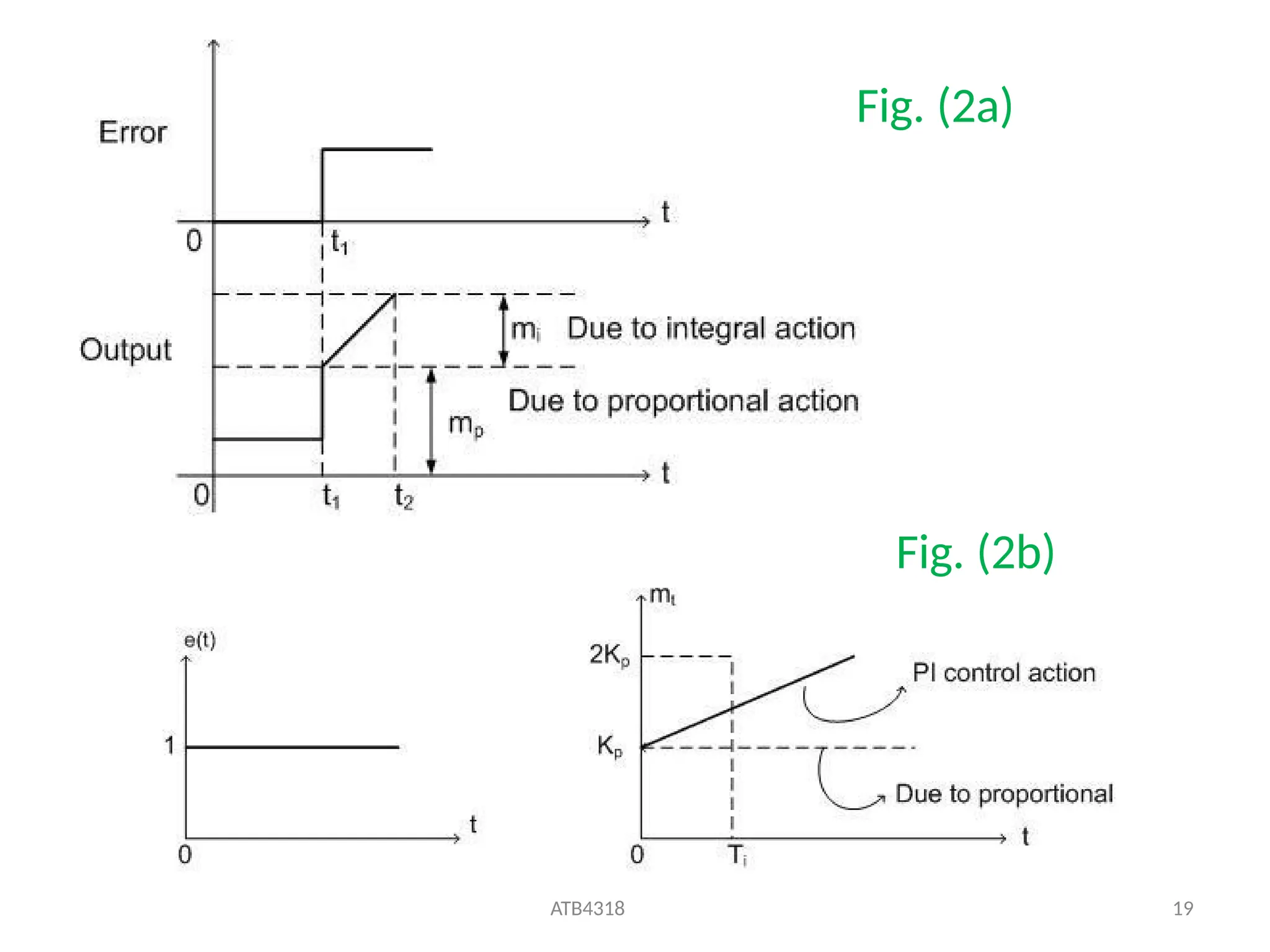
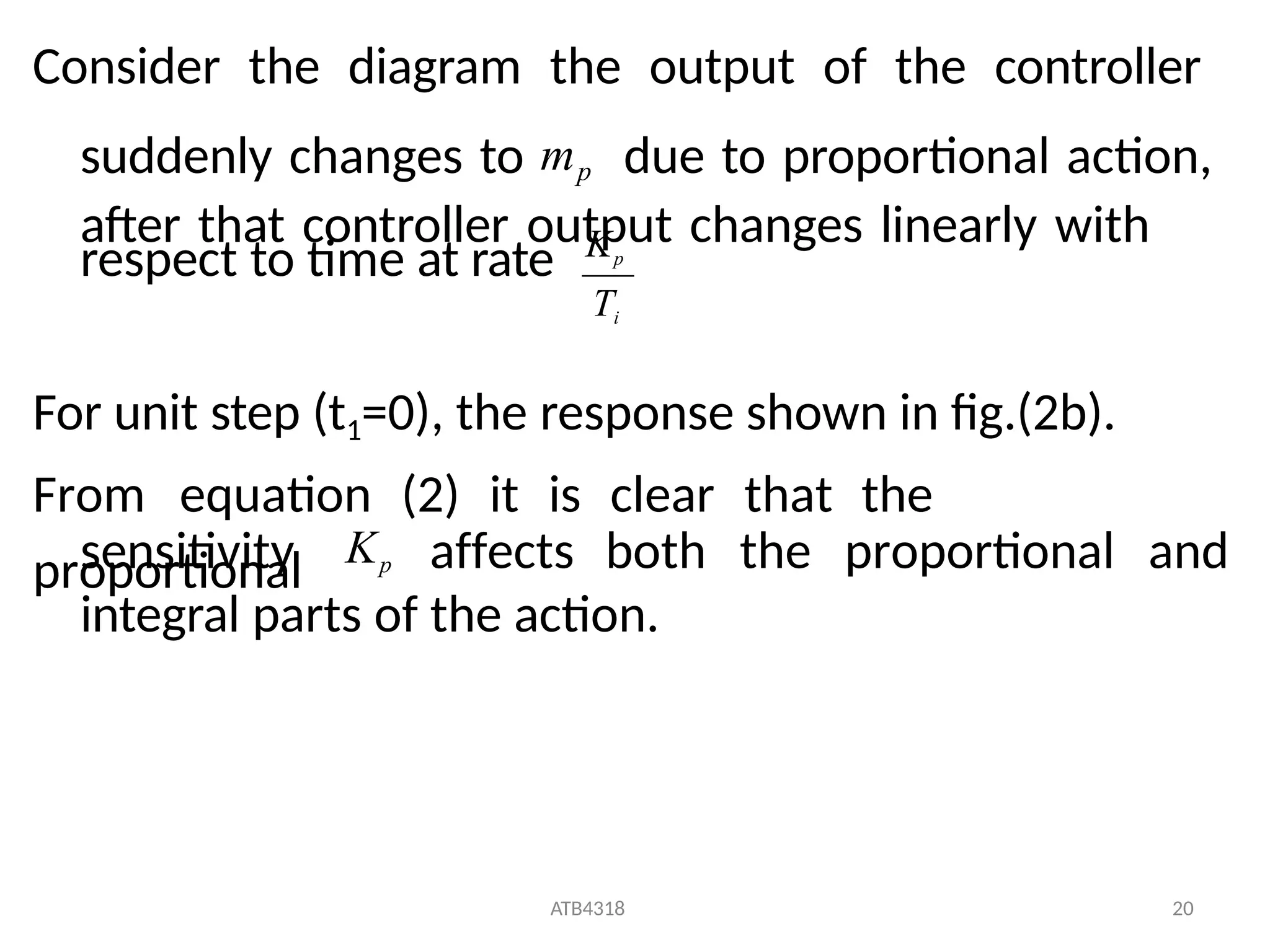
Consider the fig.(2a), the error varies at t t1
Fig. (1)
respect to timeat rate
For unit step (t1=0), the response shown in fig.(2b).
From equation (2) it is clear that the
proportional
sensitivity affects both the proportional and
integral parts of the action.
Ti
ATB4318 20
Kp
Consider the diagram the output of the controller
suddenly changes to mp due to proportional action,
after that controller output changes linearly with
Kp
97.
04/07/2025
Integral Controller
Mostof the processes we will be controlling will
have a clearly defined setpoint.
If we wish to restore the process to the setpoint after
a disturbance then proportional action alone will be
insufficient.
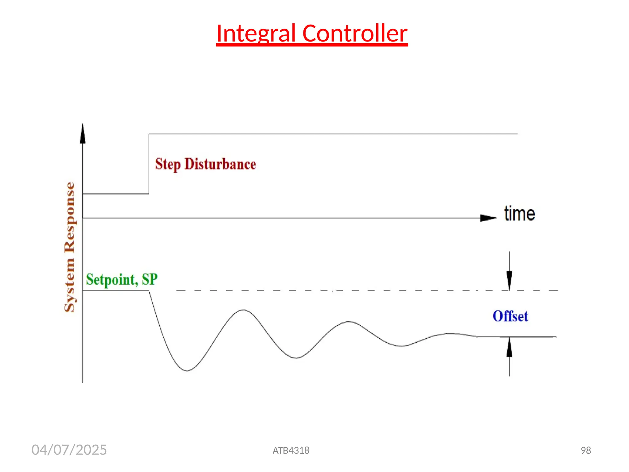
Consider the below Figure showing the response of
a system under proportional control.
ATB4318 97
04/07/2025
Integral Controller
Ifwe wish to restore the process to the setpoint we
must increase the inflow over and above that
required to restore a mass balance.
The additional inflow must replace the lost volume
and then revert to a mass balance situation to
maintain the level at the setpoint.
This is shown in below Figure.
This additional control signal must be present until
the error signal is once again zero.
ATB4318 99
04/07/2025
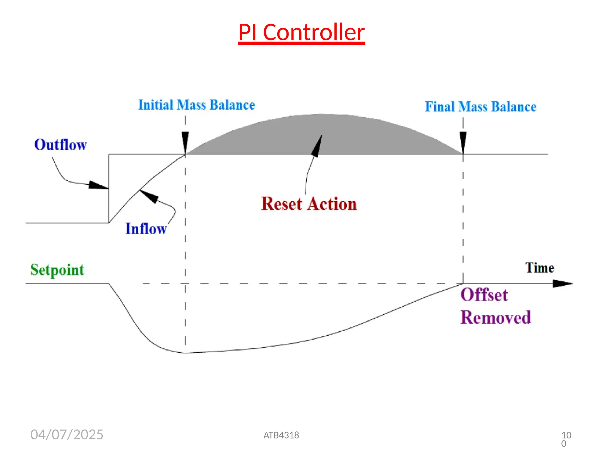
PI Controller
Thisadditional control signal is known as Reset
action, it resets the process to the setpoint.
Reset action is always used in conjunction
with proportional action.
Mathematically, reset action is the integration of
the error signal to zero hence the alternative
nomenclature Integral action.
–
The combination of proportional plus reset action is
usually referred to as PI control.
ATB4318 10
1
102.
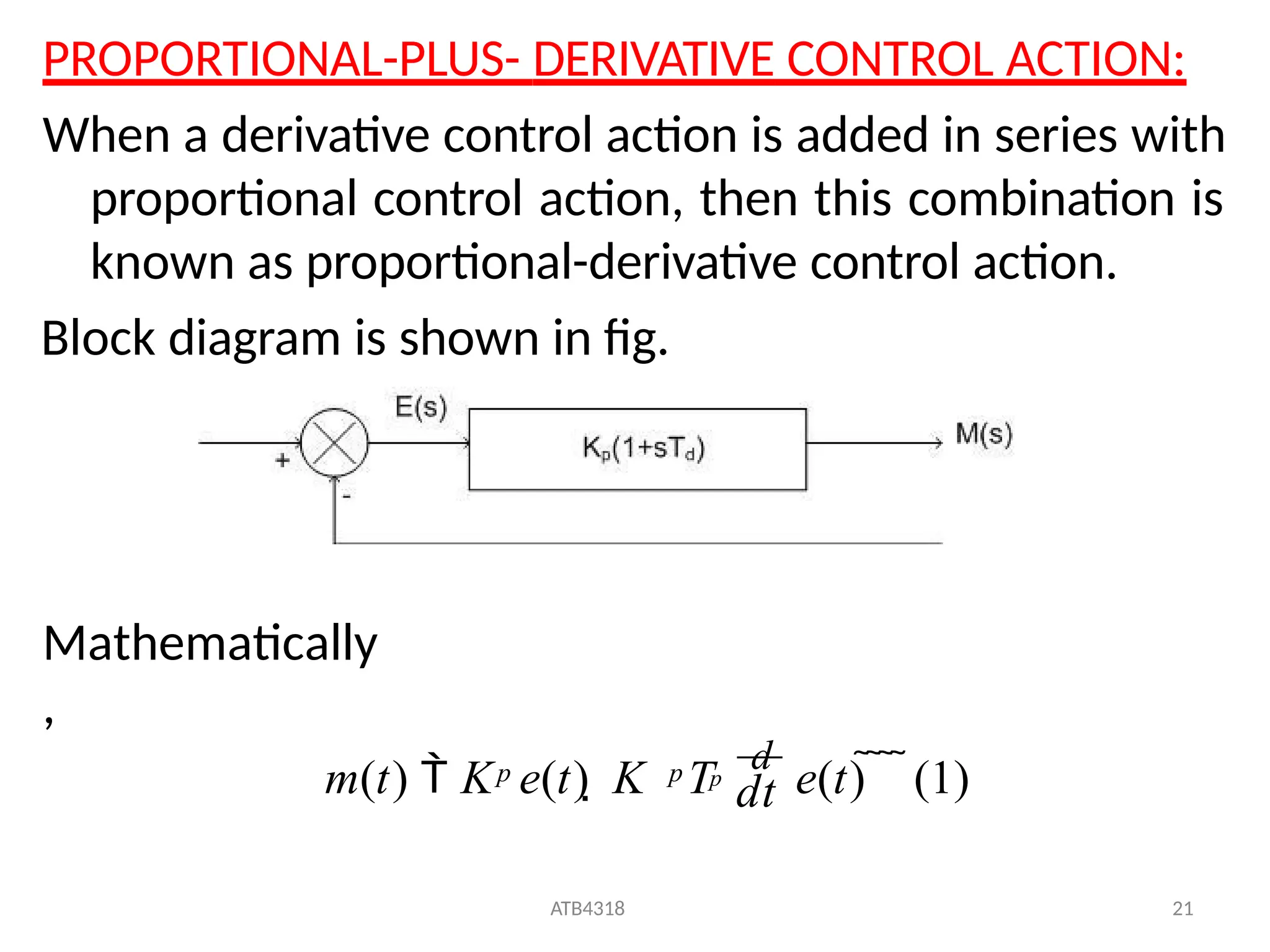
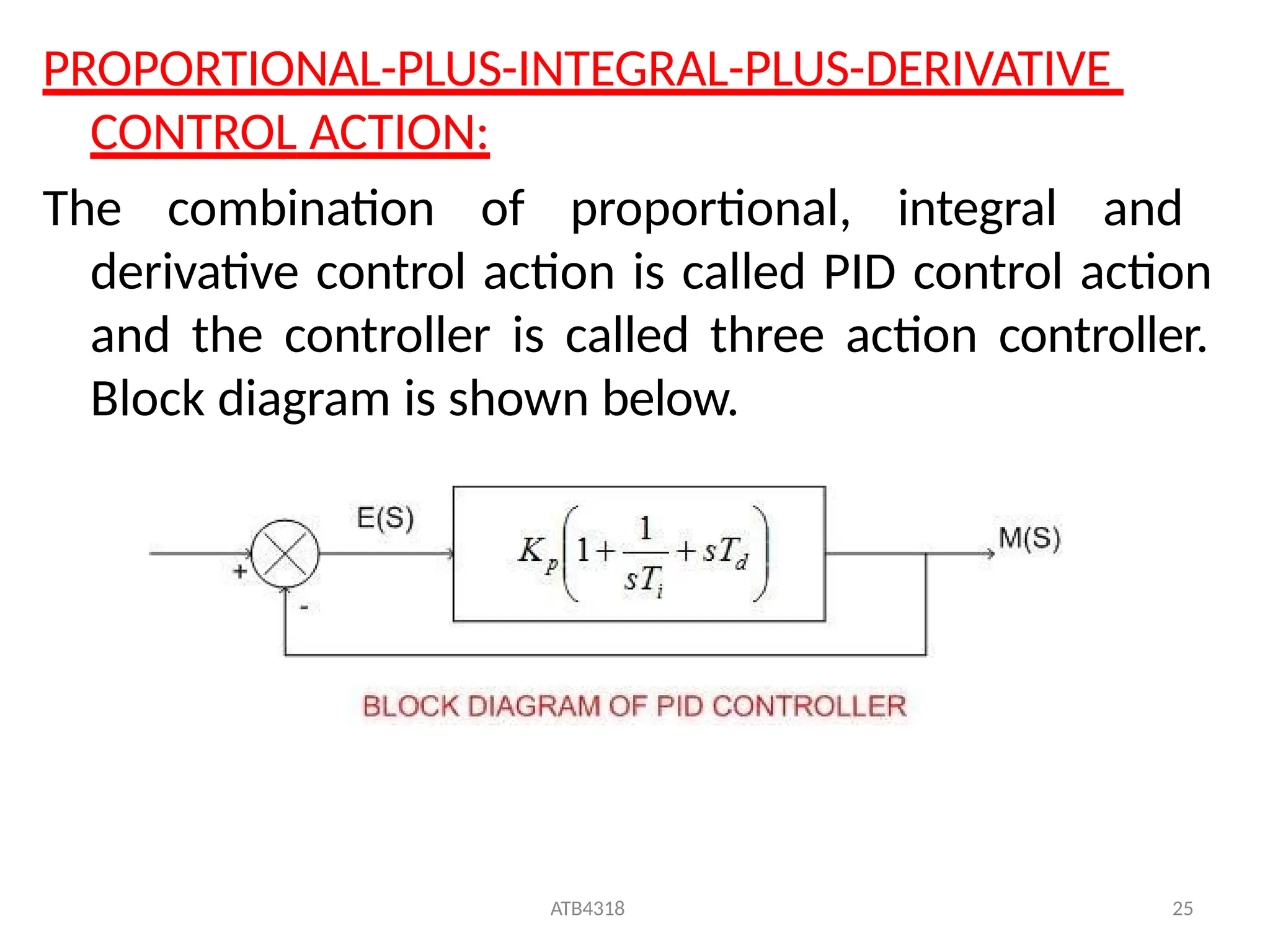
PROPORTIONAL-PLUS- DERIVATIVE CONTROLACTION:
When a derivative control action is added in series with
proportional control action, then this combination is
known as proportional-derivative control action.
Block diagram is shown in fig.
Mathematically
,
m(t) K e(t) K T
d
e(t) (1)
ATB4318 21
p
dt
p p
103.
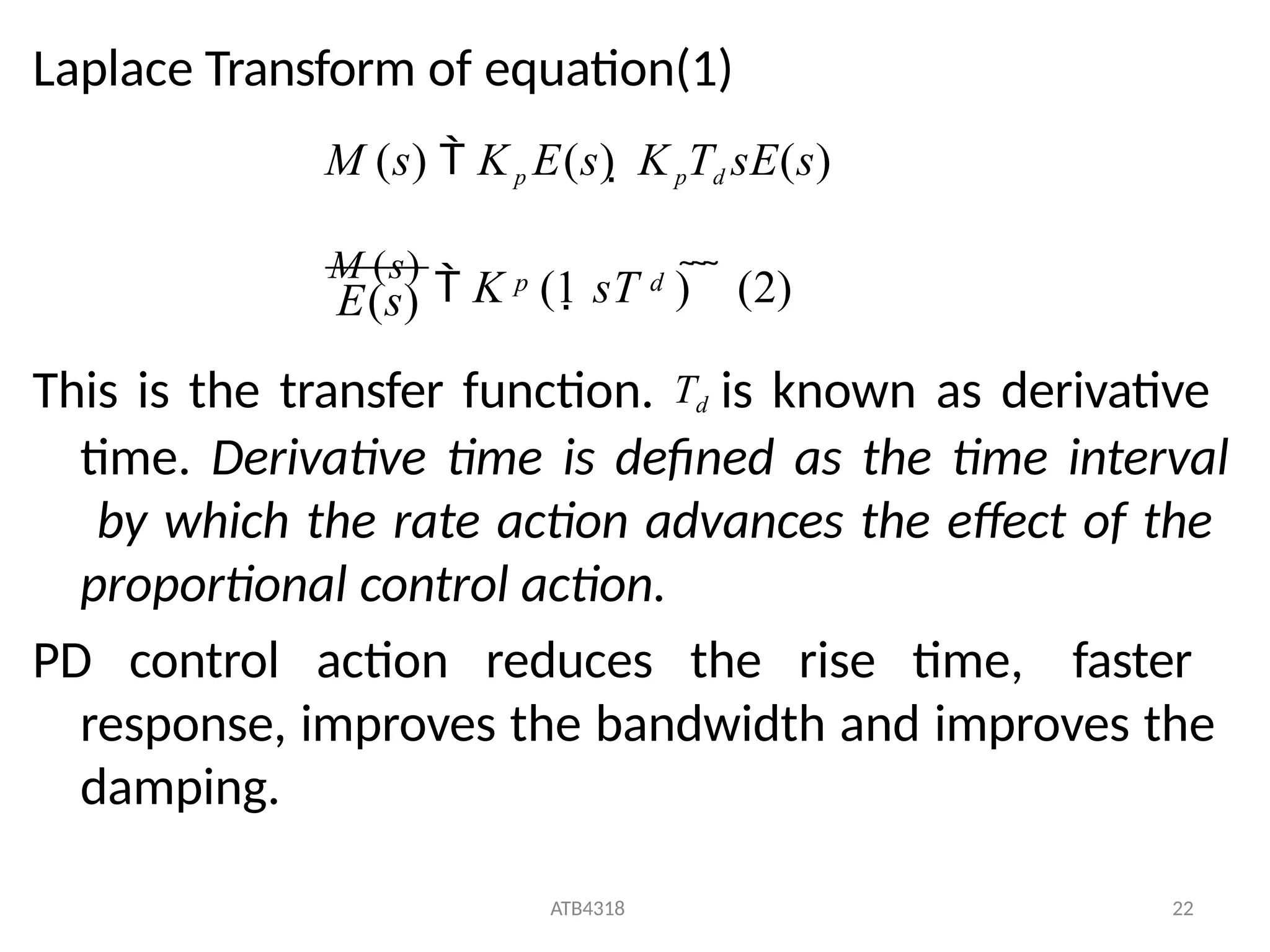
Laplace Transform ofequation(1)
This is the transfer function. Td is known as derivative
time. Derivative time is defined as the time interval
by which the rate action advances the effect of the
proportional control action.
PD control action reduces the rise time, faster
response, improves the bandwidth and improves the
damping.
M (s) Kp E(s) KpTd sE(s)
ATB4318 22
p d
E(s)
M (s)
K (1 sT ) (2)
104.
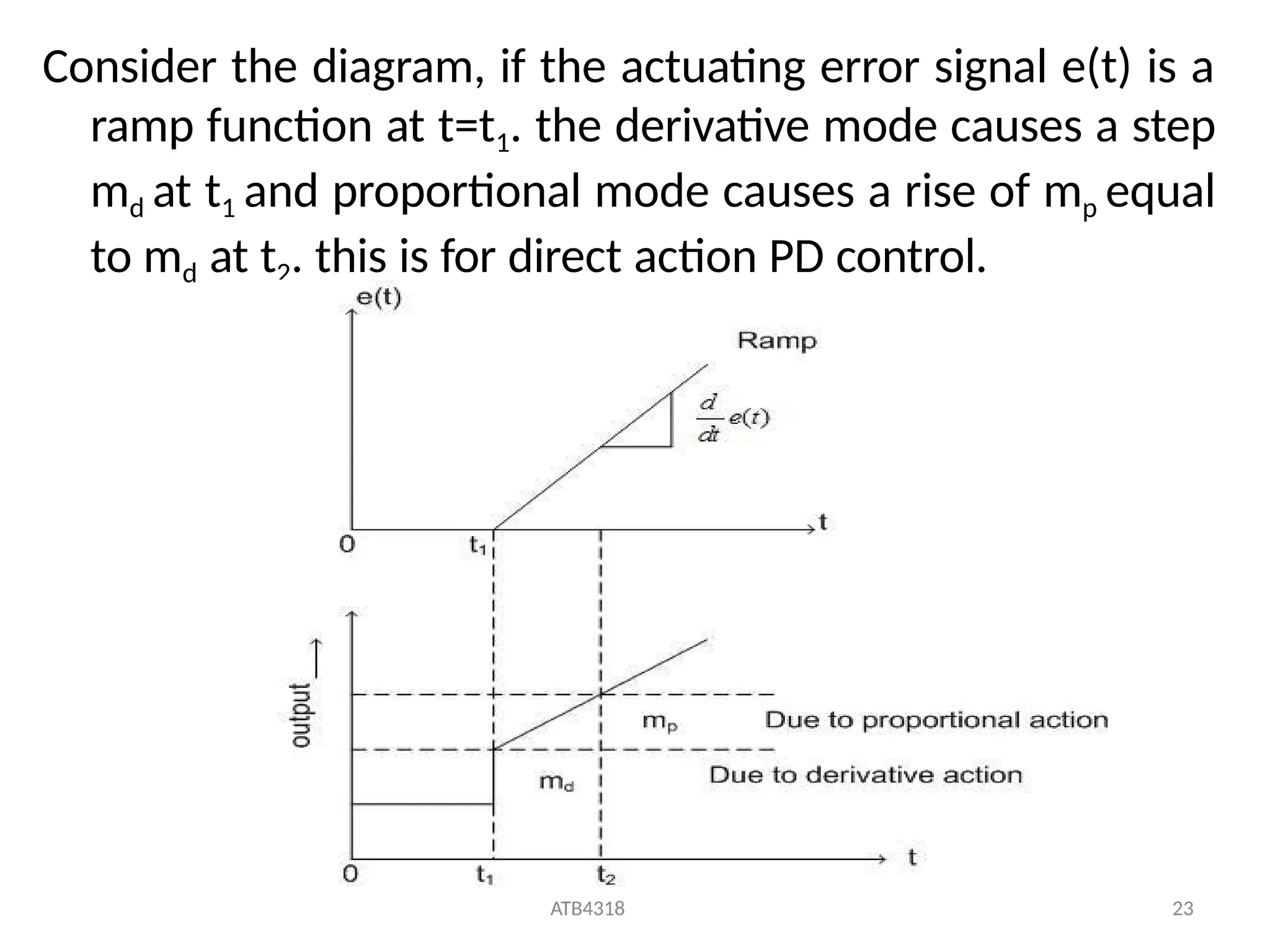
Consider the diagram,if the actuating error signal e(t) is a
ramp function at t=t1. the derivative mode causes a step
md at t1 and proportional mode causes a rise of mp equal
to md at t2. this is for direct action PD control.
ATB4318 23
105.
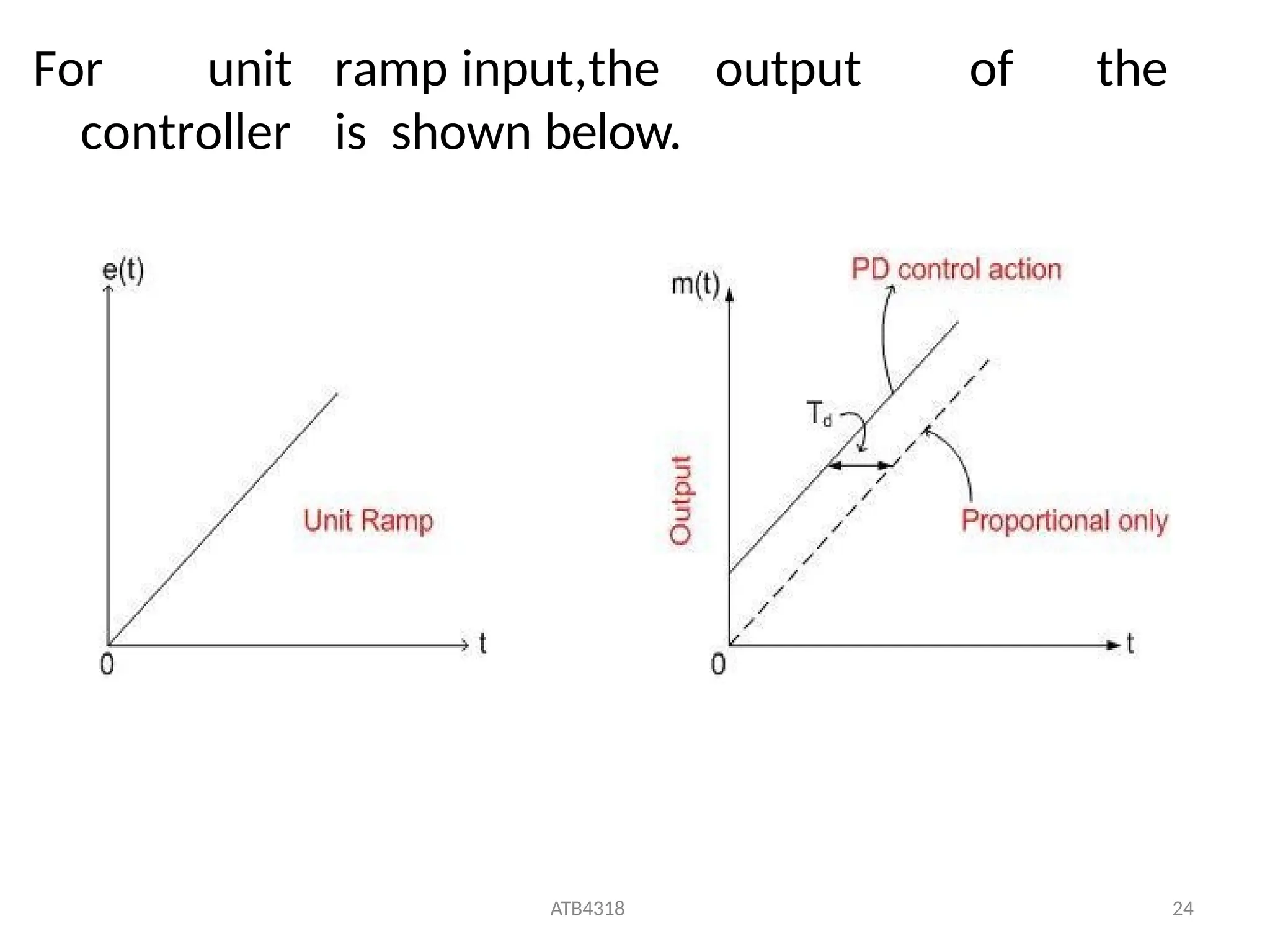
For unit rampinput,the output of the
controller is shown below.
ATB4318 24
1
ATB4318 26
E(s)
M (s)
0
d
i
p
sT (2)
p d
E(s) K T sE(s)
i
p
p
M (s) K E(s)
p d
t
i
1
T
p
p
m(t) K e(t) K
sT
K 1
sT
K
dt
e(t)dt K T
d
e(t) (1)
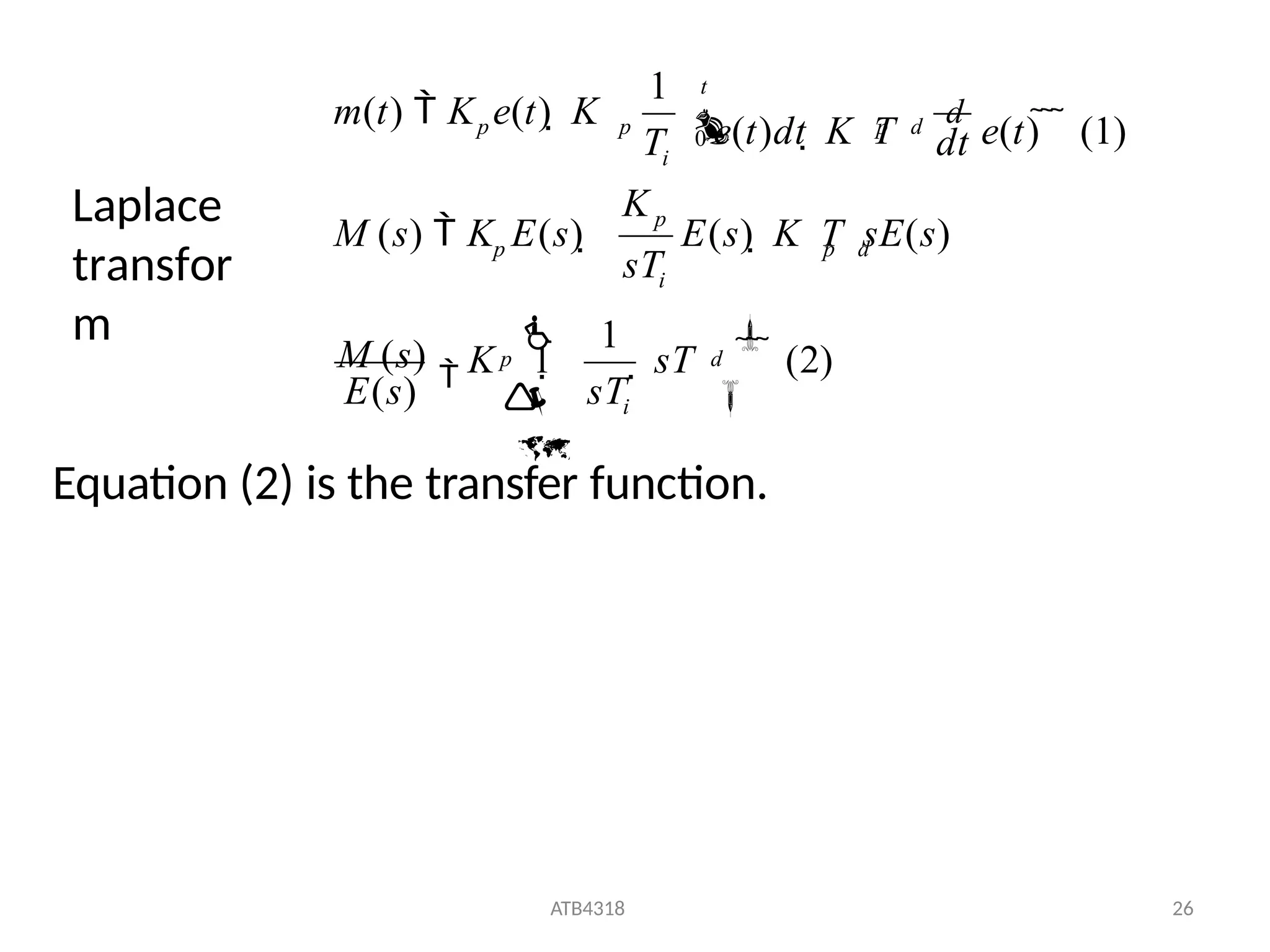
Laplace
transfor
m
Equation (2) is the transfer function.


![lcs_manual_1[1].pdf](https://cdn.slidesharecdn.com/ss_thumbnails/lcsmanual11-230906185309-7d644dc9-thumbnail.jpg?width=640&height=640&fit=bounds)


