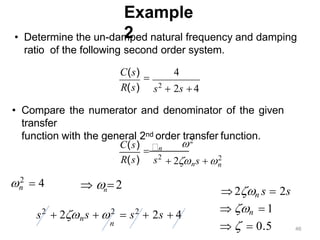
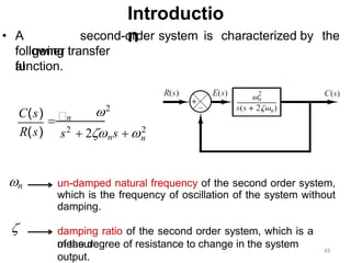
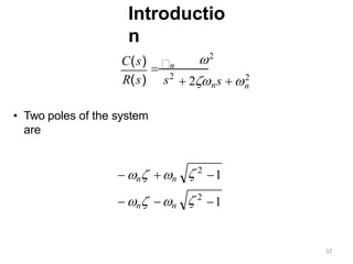
Here are the key steps: 1) Identify the second order system transfer function: C(s)/R(s) = 4/(s^2 + 2s + 4) 2) Compare to the general second order system transfer function: C(s)/R(s) = ωn^2/(s^2 + 2ζωns + ωn^2) 3) Equate coefficients: ωn^2 = 4 2ζωn = 2 ωn = 2 ζ = 1 Therefore, the un-damped natural frequency (ωn) is 2 rad/s and the damping ratio (ζ) is 1.

1. Time Domain Analysis

2. Introduction
• In time-domain analysis the response of a dynamic system to an input is expressed as a
function of time.
• It is possible to compute the time response of a system if the nature of input and the
mathematical model of the system are known.
• Usually, the input signals to control systems are not known fully ahead of time.
• It is therefore difficult to express the actual input signals mathematically by simple
equations.

3. Standard Test Signals
• The characteristics of actual input signals are a sudden shock,
a sudden change, a constant velocity, and constant
acceleration.
• The dynamic behavior of a system is therefore judged and
compared under application of standard test signals – an
impulse, a step, a constant velocity, and constant acceleration.
• The other standard signal of great importance is a sinusoidal
signal.

4. Standard Test Signals
• Impulse signal
– The impulse signal imitate the
sudden shock characteristic of
actual input signal.
– If A=1, the impulse signal is
called unit impulse signal.
0 t
δ(t)
A

t  0
0 t  0
(t) 
A

5. Standard Test Signals
• Step signal
– The step signal imitate
change
of actual
the sudden
characteristic
input signal.
– If A=1, the step signal is
called unit step signal
t  0
0 t  0
A
u(t)   0 t
u(t)
A

6. Standard Test Signals
• Ramp signal
– The ramp signal imitate
the constant velocity
characteristic of actual
input signal.
– If A=1, the ramp signal
is called unit ramp
signal

t  0
0 t  0
r(t) 
At
0 t
r(t)
r(t)
unit ramp signal
r(t)
ramp signal with slopeA

7. Standard Test Signals
• Parabolic signal
– The parabolic
imitate the
signal
constant
acceleration characteristic
of actual input signal.
signal is called unit
parabolic signal.

– If A=1, the parabolic
0
 2
t  0
t  0
 At2
p(t ) 
0 t
p(t)
parabolic signal with slopeA
p(t
)
Unit parabolic signal
p(t
)

8. Relation between standard Test Signals
• Impulse
• Step
• Ramp
• Parabolic

t  0
0 t  0
(t) 
A

t  0
0 t  0
u(t) 
A
dt

t  0
0 t  0
r(t) 
At

0
 2
 At2
p(t )  t  0
t  0


 dt
d
d
dt
d

9. Laplace Transform of Test Signals
• Impulse
• Step

t  0
0 t  0
(t) 
A
L{(t)}  (s)  A

t  0
0 t  0
u(t) 
A
S
L{u(t)} U(s) 
A

10. Laplace Transform of Test Signalst
• Ramp
• Parabolic
s2
L{r(t)}  R(s) 
A
S3
L{ p(t)} P(s) 
A
t  0
0 t  0
At
r(t)  

0
 2
 At2
p(t )  t  0
t  0

11. Time Response of Control Systems
Syste
m
• The time response of any system has two components
• Transient response
• Steady-state response.
• Time response of a dynamic system response to an
expressed as a function of time.
input

12. Time Response of Control
Systems
• When the response of the system is changed from
equilibrium it takes some time to settle down.
• This is called transient response.
2 4 6 8 14 16 18 20
0
0
1
2
3
4
5
10 12
Time (sec)
Response
6
Step Input
Transient
Response
Steady
State
Response
• The response of the
system after the
transient response is
called steady state
response.

13. Time Response of Control
Systems
• Transient response depend upon the system poles only
and not
on the type of input.
• It is therefore sufficient to analyze the transient response
using a step input.
• The steady-state response depends on system dynamics
and the input quantity.
• It is then examinedusing different test signalsby final
value theorem.

14. Introduction
• The first order system has only one pole.
C(s)

K
R(s) Ts 1
• Where K is the D.C gain and T is the time
constant of the system.
• Time constant is a measureof how quickly a
1st order system responds to a unit step
input.
• D.C Gain of the system is ratio between the
input signal and the steady state value of

15. Introduction
• The first order system given
below.
3s 1
10
G(s) 
3
G(s) 
3/ 5

s  5 1/ 5s 1
• D.C gain is 10 and time constant is 3
seconds.
• For the following system
• D.CGainof the systemis 3/5 and time constant is 1/5
seconds.

16. Impulse Response of 1st Order System
• Consider the following 1st order
system
K
Ts  1
C(s)
R(s)
0
t
δ(t)
1
R(s)  (s)  1
Ts 1
C(s) 
K

17. Impulse Response of 1st Order
System
• Re-arrange following equation
as
Ts 1
C(s) 
K
s 1/T
K /T
C(s) 
T
c(t) 
K
et / T
• In order to compute the response of the system in time
domain we need to compute inverse Laplace transform of
the above equation.
C

  Ceat

 
s  a
L1

18. Impulse Response of 1st Order
System c(t) 
K
et / T
T
K/T*exp(-t/T)
• If K=3 and T=2s
then
0
0 2 4 6 8 10
0.5
1
1.5
Time
c(t)

19. Step Response of 1st Order
System
• Consider the following 1st order
system
K
Ts  1
C(s)
R(s)
R(s)  U(s)
1
s
 
s Ts 1
C(s) 
K
s Ts 1
C(s) 
K

KT
• In order to find out the inverse Laplace of the above equation,
we need to break it into partial fraction expansion (page
867 in the
T
extbook
)

20. Step Response of 1st Order
System
• Taking Inverse Laplace of above
equation

T
 
 s Ts 1
C(s)  K 1

c(t)  Ku(t)  et /T

c(t)  K1 et /T

• Where
u(t)=1
• When t=T (time constant)
c(t)  K1
 e1
 0.632K

21. Step Response of 1st Order System
• If K=10 and T=1.5s
then
c(t)  K1
 et /T

K*(1-exp(-t/T))
0
0 1 2 3 4 6 7 8 9 10
5
Time
1
5
4
3
2
6
7
8
9
11
10
c(t)
Unit Step Input
Step Response
Input 1
D.C Gain  K 
steady state output

10
63
%

22. Step Response of 1st order System
• System takes five time
constantsto reach its final
value.

23. Step Response of 1st Order System
• If K=10 and T=1, 3,
5, 7
c(t)  K1
 et /T

K*(1-exp(-t/T))
8
7
6
5
4
3
2
1
0
0 5 10 15
Time
11
10
9
c(t)
T=3s
T=5s
T=7s
T=1s

24. Step Response of 1st Order System
• If K=1, 3, 5, 10 and
T=1
c(t)  K1
 et /T

K*(1-exp(-t/T))
11
10
9
8
7
6
5
4
3
2
1
0
0 5 10 15
Time
c(t)
K=1
K=3
K=5
K=10

25. Ramp Response of 1st Order System
• Consider the following 1st order
system
K
Ts  1
C(s)
R(s)
s2
R(s) 
1
K
s2
Ts1
C(s) 
• The ramp response is given as
c(t)  Kt T  Tet / T


26. Parabolic Response of 1st Order System
• Consider the following 1st order
system
K
Ts  1
C(s)
R(s)
1
s3
R(s) 
K
s3
Ts1
C(s) 
Therefore
,

27. Practical Determination of Transfer
Function of 1st Order Systems
• Often it is not possible or practical to obtain a system's
transfer function analytically.
• Perhaps the system is closed, and the component parts
are not easily identifiable.
• The system's step response can lead to a representation
even though the inner construction is not known.
• With a step input, we can measure the time constant and
the steady-state value, from which the transfer function
can be calculated.

28. Practical Determination of Transfer
Function of 1st Order Systems
• If we can identify T and K empirically we can obtain
the transfer function of the system.
C(s)

K
R(s) Ts 1

29. Practical Determination of Transfer Function
of 1st Order Systems
• For example, assume the unit
step response given in
figure.
• From the response, we can
measure the time constant,
that is, the time for the
amplitude to reach 63% of its
final value.
• Since the final value is about
0.72 the time constant is
evaluated where the
curve
reaches0.63 x 0.72 = 0.45, or
about 0.13 second.
• K is simply steady state value.
T=0.13
s
K=0.72
function is

s 7.7
• Thus transfer
obtained as:
C(s)

0.72 5.5
R(s) 0.13s 1

30. First Order System with a Zero
C(s)

K(1s)
R(s) Ts 1
• Zero of the system lie at -1/α and pole at -
1/T.
• Step response of the system would be:
C(s) 
K(1s)
sTs1
C(s) 
K

K(  T)
s Ts 1
T
c(t )  K 
K
(  T )et /T

31. First Order System With
Delays
• Following transfer function is the generic
representation of 1st order system with time
lag.
• Where td is the delay
time.
estd
C(s)

K
R(s) Ts 1

32. First Order System With
Delays
estd
C(s)

K
R(s) Ts 1
1
Unit Step
Step
Response
t
td

33. First Order System With
Delays
[10(t  2) 10e1/3(t2)
]u(t  2)
4
2
10 10
L1
[es
F(s)]  f (t  )u(t  )
s(3s1)
10
C(s) 
R(s) 3s1
C(s)

10
e2s
1
)e ]
s s 1/ 3
L [(  2s
e2s
0 5 10 15
0
6
8
10
Step Response
Time (sec)
td2s
T3s
K10

34. Second Order
System
• We have already discussed the affect of location of poles and
zeros on the transient response of 1st order systems.
• Compared to the simplicity of a first-order system, a second-order
system
exhibits a wide range of responses that must be analyzed and
described.
• Varying a first-order system's parameter (T, K) simply changes the
speed
and offset of the response
• Whereas,changesin the parameters of a second-ordersystem
can change the form of the response.
oscillations for its transient 44

35. Introductio
n
• A
gener
al
second-order system is characterized by the
following transfer
function.
n
2
s2
 2ns  2
n
R(s)
C(s)
45
un-damped natural frequency of the second order system,
which is the frequency of oscillation of the system without
damping.
n
damping ratio of the second order system, which is a
measure
of the degree of resistance to change in the system
output.


36. Example
2
s2
 2s  4
• Determine the un-damped natural frequency and damping
ratio of the following second order system.
C(s)

4
R(s)
n
2
 4
n
s2
2
 2ns  2
n
R(s)
C(s)
• Compare the numerator and denominator of the given
transfer
function with the general 2nd order transfer function.
n
   2
 2n s  2s
 n  1
   0.5
s2
 2ns  2
 s2
 2s  4
n
46

37. Introductio
n
n
s2
2
 2ns  2
n
R(s)
C(s)
• Two poles of the system
are
1
37
1
 2
 2
 n n
 n n

38. Introductio
n
• According the value of  , a second-order system can be set
into
one of the four categories (page 169 in the textbook):
1. Overdamped - when the system has two real distinct
poles ( 
1
1
 2
 2
 n n
 n n
>1)
.
-
a
-b
-
c
δ
j
ω
38

39. Introductio
n
• According the value of  , a second-order system can be set
into one of the four categories (page 169 in the textbook):
2. Underdamped - when the system has two complex conjugate poles (0
< <1)
jω
1
1
 2
 2
 n n
 n n
-
a
-b
-
c
δ
39

40. Introductio
n
• According the value of  , a second-order system can be set
into one of the four categories (page 169 in the textbook):
1
1
 2
 2
 n n
 n n
3. Undamped - when the system has two imaginary
poles ( 
jω
=
0).
-
a
-b
-
c
δ
40

41. Introductio
n
• According the value of  , a second-order system can be set
into one of the four categories (page 169 in the textbook):
1
1
 2
 2
 n n
 n n
4. Critically damped - when the system has two real but equal
poles (
jω
=
1).
-
a
-b
-
c
δ
41

42. Underdamped
System
For 0<  <1 and ωn > 0, the 2nd order system’s response
due to a unit step input is as follows.
Important timing characteristics: delay time, rise time,
peak time, maximum overshoot, and settling time.
42

43. Delay
Time
• The delay (td) time is the time required for the
response to reach half the final value the very first
time.
43

44. Rise
Time
• The rise time is the time required for the response to rise from
10% to 90%, 5% to 95%, or 0% to 100% of its final value.
• For underdamped second order systems, the 0% to 100% rise
time is normally used. For overdamped systems, the 10% to
90% rise time is commonly used.

45. Peak
Time
• The peak time is the time required for the response to
reach the first peak of the overshoot.
55
45

46. Maximum
Overshoot
The maximum overshoot is the maximum peak value of the
response curve measured from unity. If the final steady-
state value of the response differs from unity, then it is
common to use the maximum percent overshoot. It is
defined by
The amount of the maximum (percent) overshoot
directly indicates the relative stability of the system.
46

47. Settling
Time
• The settling time is the time required for the response
curve to reach and stay within a range about the final
value of size specified by absolute percentage of the
final value (usually 2% or 5%).
47

48. Step Response of underdamped
System
s2
 2ns   2
2
 2
 2
2
n n n
s  2n
C(s) 
1

s
• The partial fraction expansion of above equation is
given as
s  2n
C(s) 
1

s n
s2
 2ns  2
2
n
s  2 
2

1  
2
n
2
2
1 
C(s) 
1

s n
s n 2
  
s  2n
n
s2
2
 2ns  2
n
R(s)
C(s)
2
2
n
n
2
ss  2 s   
C(s) n
Step
Response
58

49. Step Response of underdamped
System
• Above equation can be written
as
2
2
1 
C(s) 
1

s n
s n 2
  
s  2n
d
s  2n
s n 2
 2
C(s) 
1

s
d  n 1  2
• Wher
e
, is the frequency of transient
oscillations
and is called damped natural frequency.
• The inverse Laplace transform of above equation can be
obtained easily if C(s) is written in the following form:
2
2
2
2
C(s) 
1

s d
n
d
n s    

s    
s n n
59

50. Step Response of underdamped
System
2
2
2
2
C(s) 
1

s d
n
d
n s    

s    
s n n
2
1
s n d
n
d
s  n 2
 2
s 
n 
C(s) 
 
s     2
1  2
1  2
C(s) 
1

s d
d
s  n 2
 2
d
s  n
s  n 2
 2


d
50
d
cos t  n
1  2

e sin  t
 t
n
 t
c(t)  1 e
1  2

51. Step Response of underdamped
System
d
d
cos t  n
e sin  t
 t
n
 t
c(t)  1 e
1  2




sind t



cosd t 
1  2
n
 t
c(t)  1 e

d  n
 n
51
1  2
• When   0
c(t)  1
cosnt

52. Step Response of underdamped
System

 
 
n

 t cosd t  sind t
1  2
c(t)  1 e

and n  3
if  0.1
1.8
1.6
1.4
1.2
1
0.8
0.6
0.4
0.2
52
0
0 2 4 6 8 10

53. Step Response of underdamped
System

 
 
n

 t cosd t  sind t
1  2
c(t)  1 e

and n  3
if  0.5
1.4
1.2
1
0.8
0.6
0.4
0.2
53
0
0 2 4 6 8 10

54. Step Response of underdamped
System

 
 
n

 t cosd t  sind t
1  2
c(t)  1 e

and n  3
if  0.9
1.4
1.2
1
0.8
0.6
0.4
0.2
64
0
0 2 4 6 8 10

55. Step Response of underdamped
System

 

 
n

 t cosd t  sind t
1  2
c(t)  1 e
55

56. S-Plane (Underdamped
System)

2
 2
 n  n  1
 n  n 1
Since 𝜔2𝜁2 − 𝜔2 𝜁2− 1 = 𝜔2, the
distance from the pole to the origin is 𝜔
and 𝜁
= 𝑐
𝑜
𝑠
𝛽
56

57. Analytical
Solution
• Page 171 in the
textbook
• Rise time: set c(t)=1, we
have 𝑡
𝑟 = 𝜋−𝛽
𝜔𝑑
𝑝
• Peak time: set 𝑑𝑐(𝑡)
= 0, we have 𝑡 =
𝜋
𝜔𝑑
𝑑
𝑡
• Maximum overshoot: M𝑝 = 𝑐𝑡
𝑝 − 1 =
𝑒−(𝜁𝜔/𝜔𝑑)𝜋 (for unity output)
• Settling time: the time for the outputs
always
within 2% of the final value is
approximately
4
𝜁
𝜔






 t
c(t)  1 e n cosd t 

sind t
1 2
   1  2
n
d

58. Empirical Solution Using
MATLAB
• Page 242 in the
textbook

59. Steady State
Error
• If the output of a control system at steady state does not
exactly match with the input, the system is said to have
steady state error
• Any physical control system inherently suffers steady-
state error in response to certain types of inputs.
• Page 219 in the textbook
• A system may have no steady-state error to a step input,
but the same system may exhibit nonzero steady-state
error to a ramp input.

60. Classification of Control
Systems
• Control systems may be classified
according to their ability to follow step
inputs, ramp inputs, parabolic inputs, and
so on.
• The magnitudes of the steady-state errors
due to these individual inputs are indicative
of the goodness of the system.

61. Classification of Control
Systems
• Consider the unity-feedback control
system with the following open-loop
transfer function
• It involves the term sN in the
denominator, representing N poles at the
origin.
• A system is called type 0, type 1, type 2, ... ,
if N=0, N=1, N=2, ... , respectively.

62. Classification of Control
Systems
• As the type number is increased,accuracy
is improved.
• However, increasing the type
number aggravates the stability problem.
• A compromisebetween steady-state
accuracy and relative stability is always
necessary.

63. Steady State Error of Unity Feedback
Systems
• Consider the system shown in following
figure.
• The closed-loop transfer
function is

64. Steady State Error of Unity Feedback
Systems
input signal R(s)
is
E(s)

1
• Steadystate error is defined as the error between
the input signal and the output signal when 𝑡
→∞.
• The transfer function between the error signal E(s) and
the R(s) 1 G(s)
• The final-value theorem provides a convenient way to
find
the steady-state performance of a stable system.
• Since E(s) is
• The steady state error is

65. Static Error
Constants
• The static error constants are figures of merit of
control systems. The higher the constants, the
smaller the steady-state error.
• In a given system, the output may be the
position, velocity, pressure, temperature, or the
like.
• Therefore, in what follows, we shall call the
output “position,” the rate of change of the
output “velocity,” and so on.
• This means that in a temperature control system
“position” represents the output temperature,
“velocity” represents the rate of change of the
output temperature, and so on.

66. Static Position Error Constant
(Kp)
• The steady-state error of the system for a unit-step
input is
• The static position error constant Kp is
defined by
• Thus, the steady-state error in terms of the static
position error constant Kp is given by

67. Static Position Error Constant
(Kp)
• For a Type 0
system
• For Type 1 or higher order
systems
• For a unit step input the steady state error
ess is

68. • The steady-state error of the system for a unit-ramp
input is
• The static velocity error constant Kv is
defined by
• Thus, the steady-state error in terms of the static
velocity error constant Kv is given by
Static Velocity Error Constant
(Kv)

69. Static Velocity Error Constant
(Kv)
• For a Type 0
system
• For Type 1
systems
• For type 2 or higher order
systems

70. Static Velocity Error Constant
(Kv)
• For a ramp input the steady state error
ess is

71. • The steady-state error of the system for parabolic
input is
• The static acceleration error constant Ka is
defined by
• Thus,the steady-stateerror in terms of the static
acceleration
error constant Ka is given by
Static Acceleration Error Constant
(Ka)

72. Static Acceleration Error Constant
(Ka)
• For a Type 0
system
• For Type 1
systems
• For type 2
systems
• For type 3 or higher order
systems

73. Static Acceleration Error Constant
(Ka)
• For a parabolic input the steady state error
ess is

74. Summar
y

75. Example
2
• For the system shown in figure below evaluate the
static error constants and find the expected steady
state errors for the standard step, ramp and
parabolic inputs.
C(
S)
R(
S)
-
s2
(s  8)(s 12)
100(s  2)(s  5)

76. Example
2
G(s) 
100(s  2)(s  5)
s2
(s  8)(s 12)
s0
Kp  lim G(s)

2
100(s  2)(s  5) 
s0  s (s  8)(s 12) 
K p  lim
K p  
v lim
s0
K  sG(s)

2
100s(s  2)(s  5) 
Kv  lim
s0  s (s  8)(s 12) 
Kv  
a
K  lims2
G(s)
s0



2
s (s  8)(s 12) 
100s2
(s  2)(s  5) 
s0 
Ka  lim 
  10.4
(0  8)(0 12) 

100(0  2)(0  5) 
a
K  

77. Example
2
K p   Kv   Ka 10.4
 0
 0
 0.09