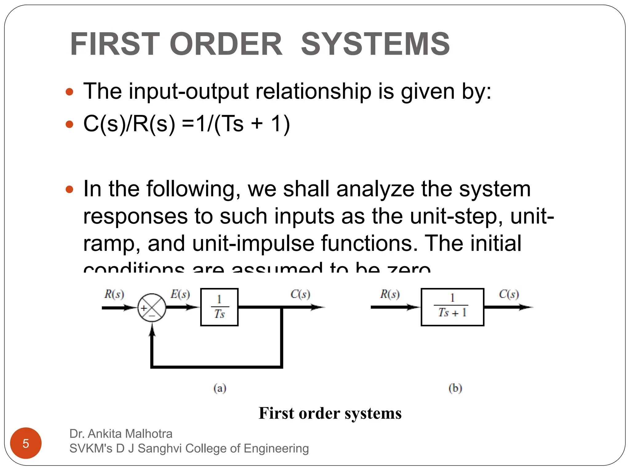
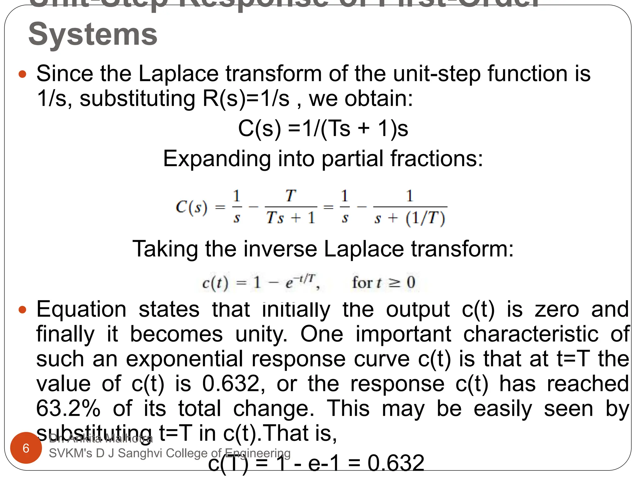
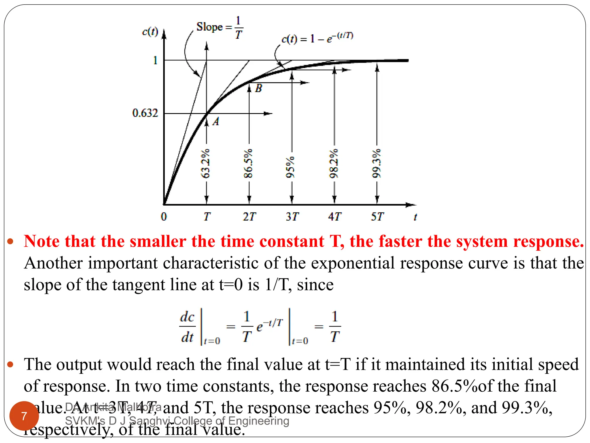
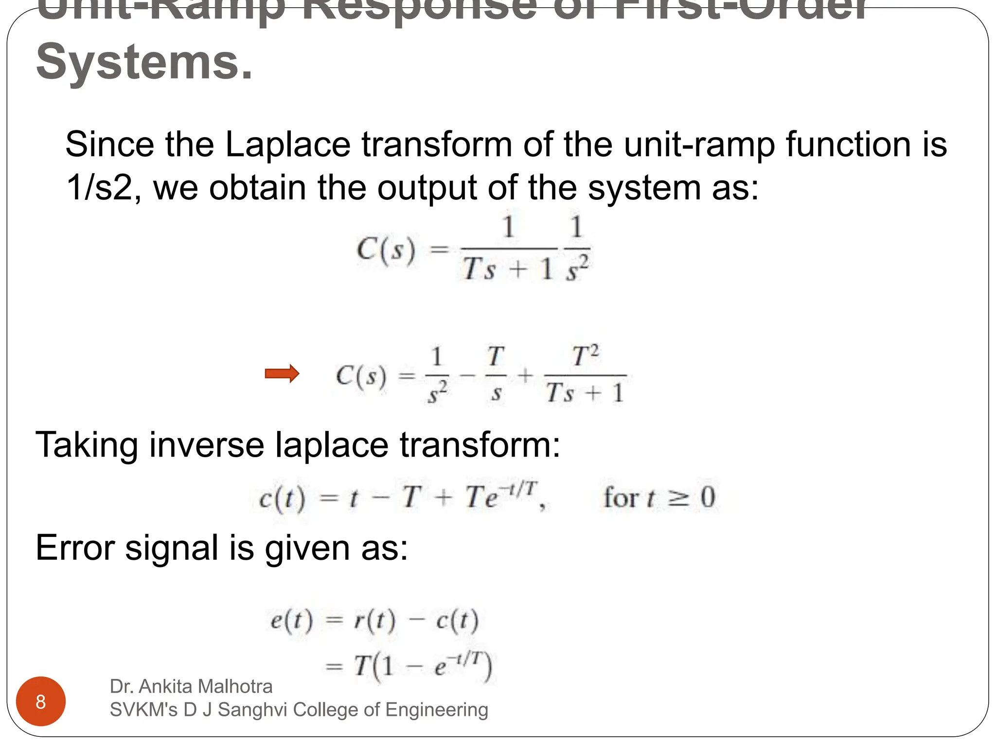
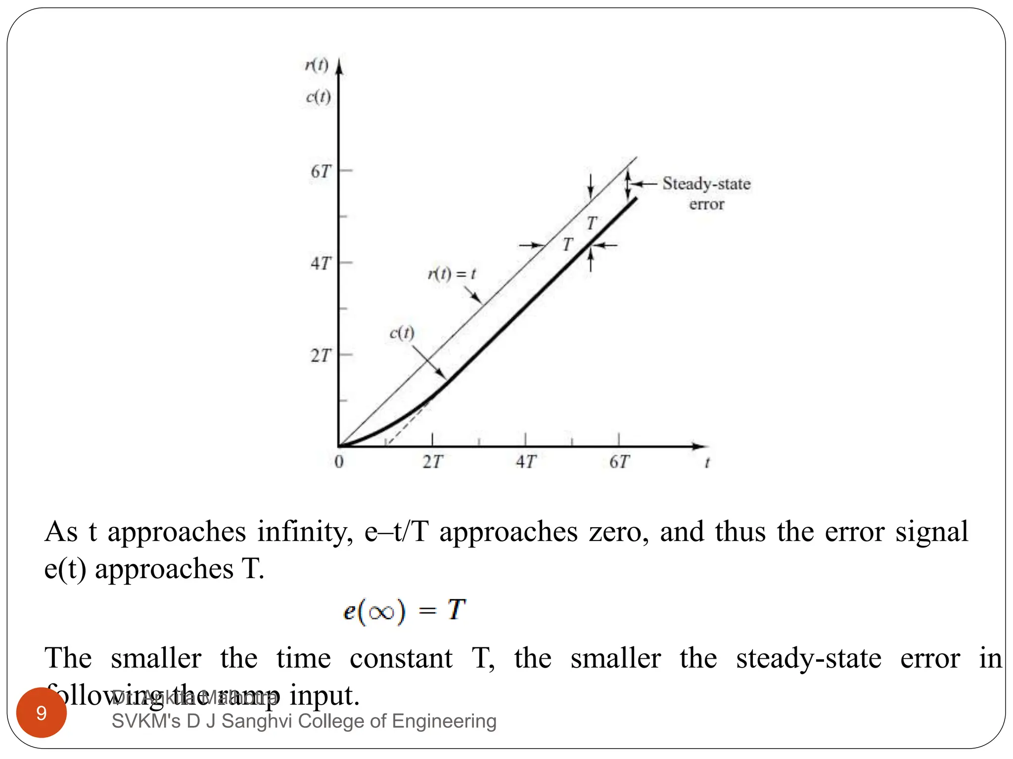
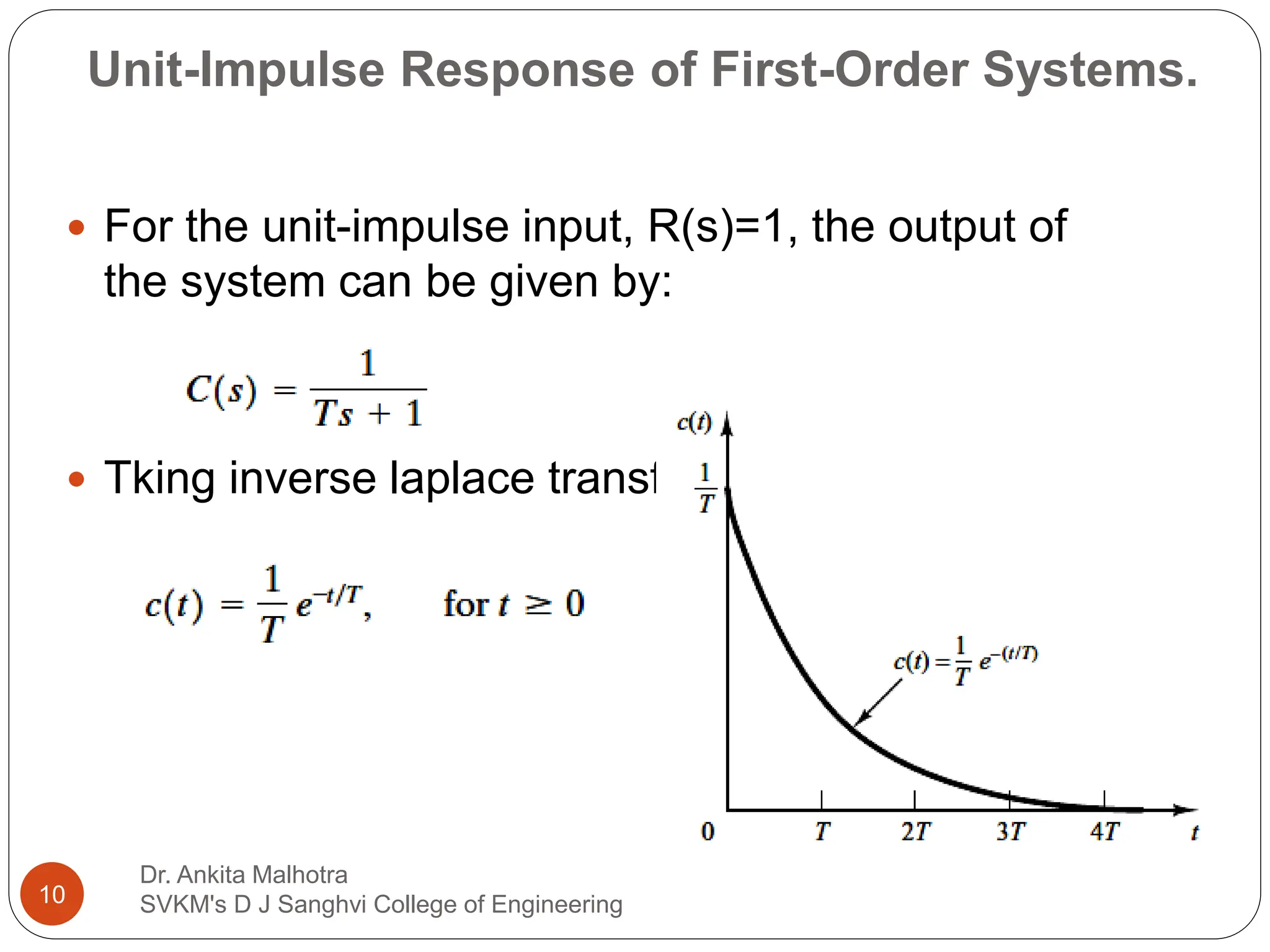
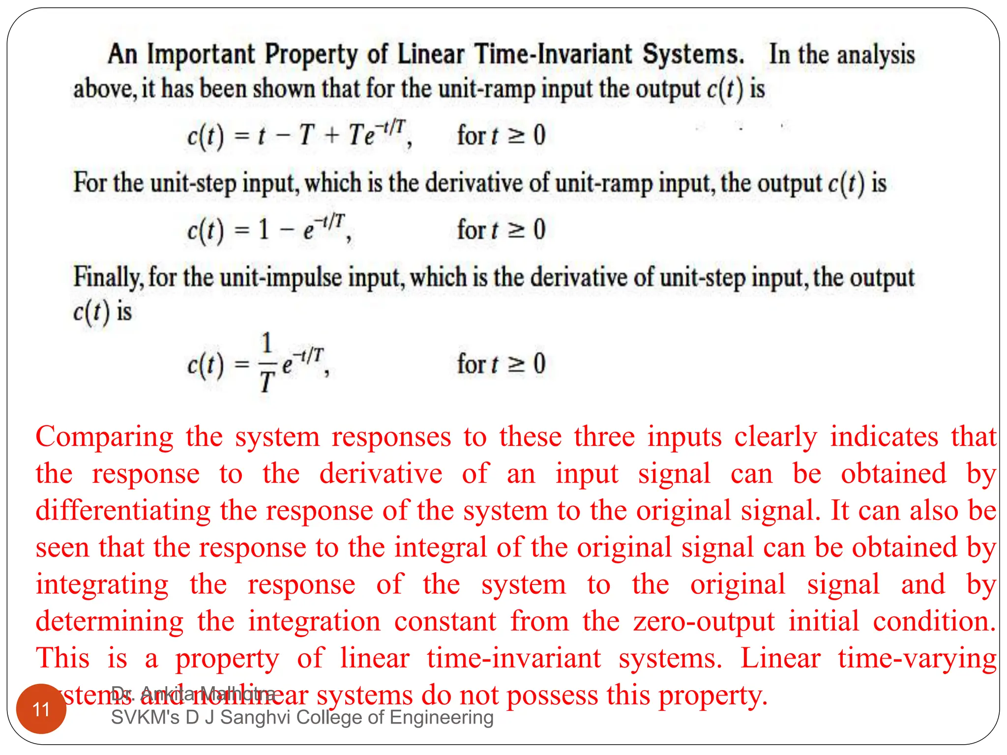
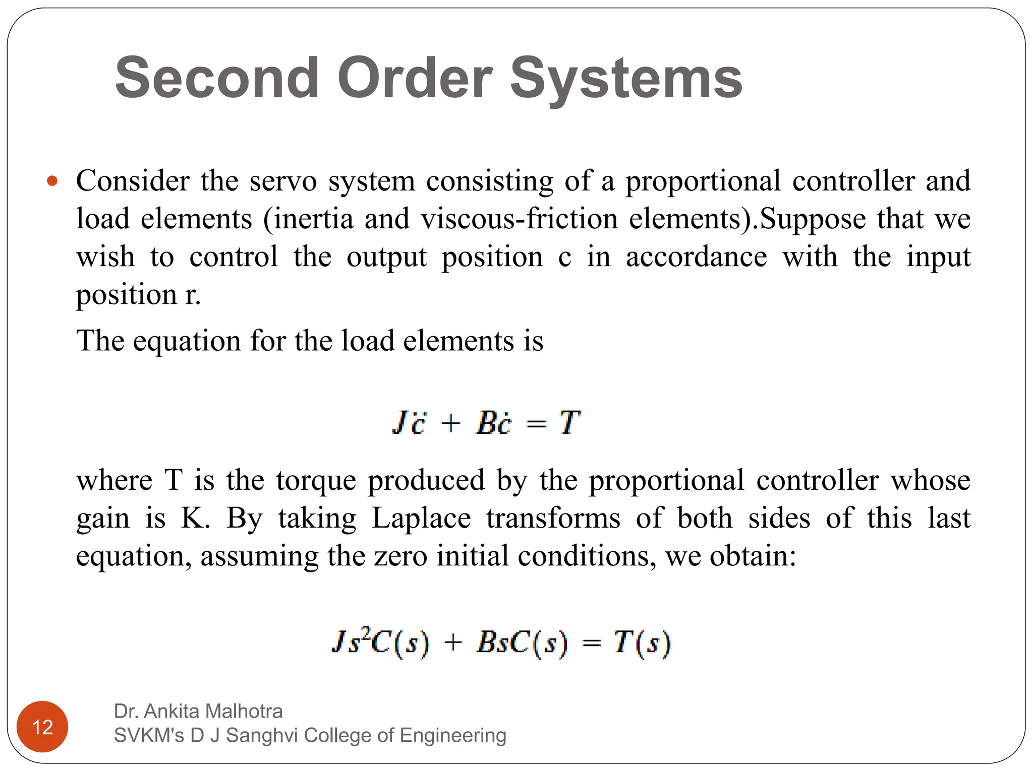
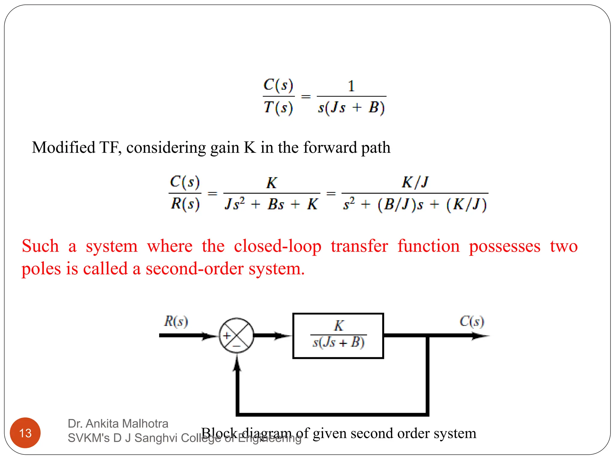
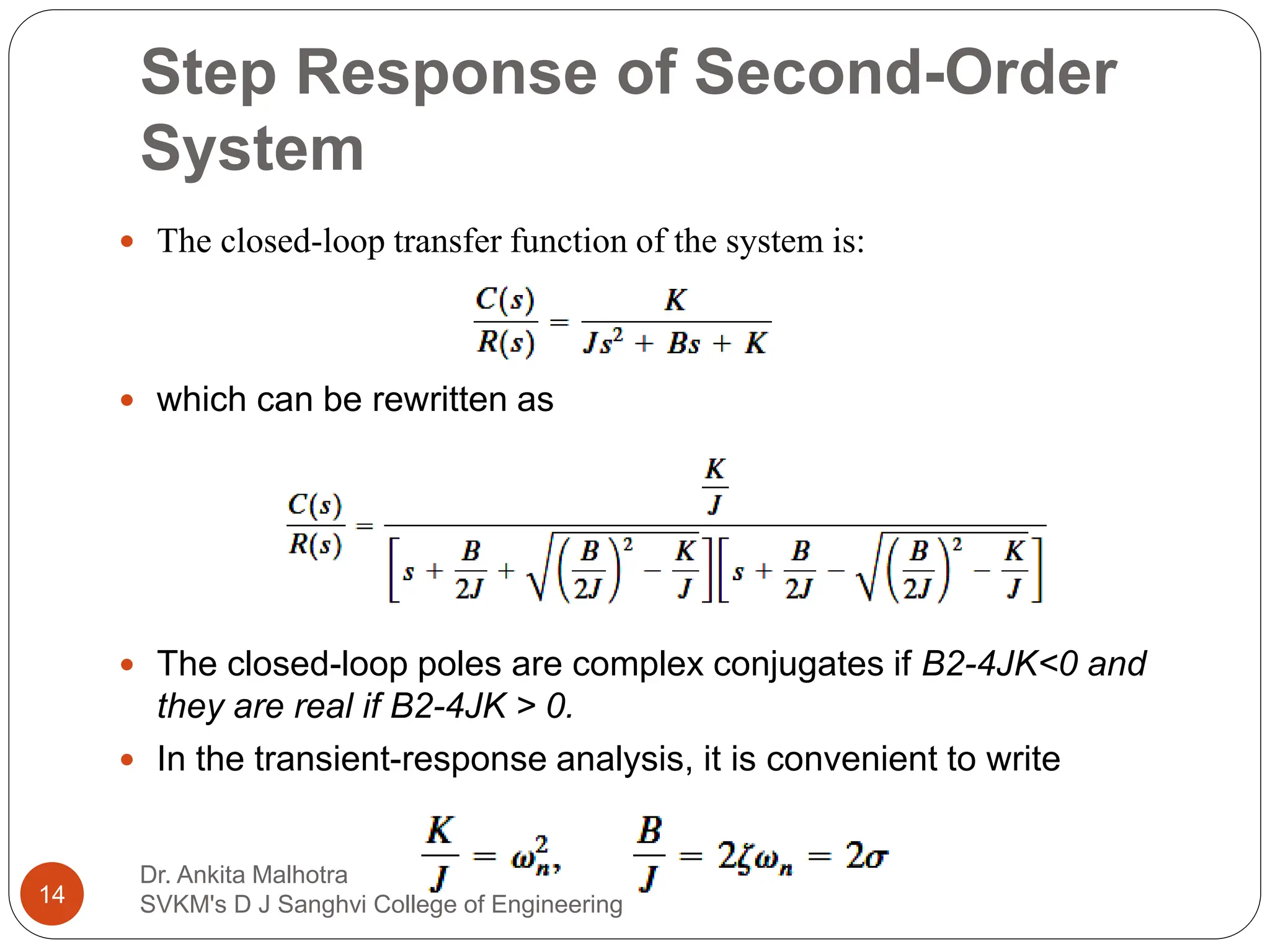
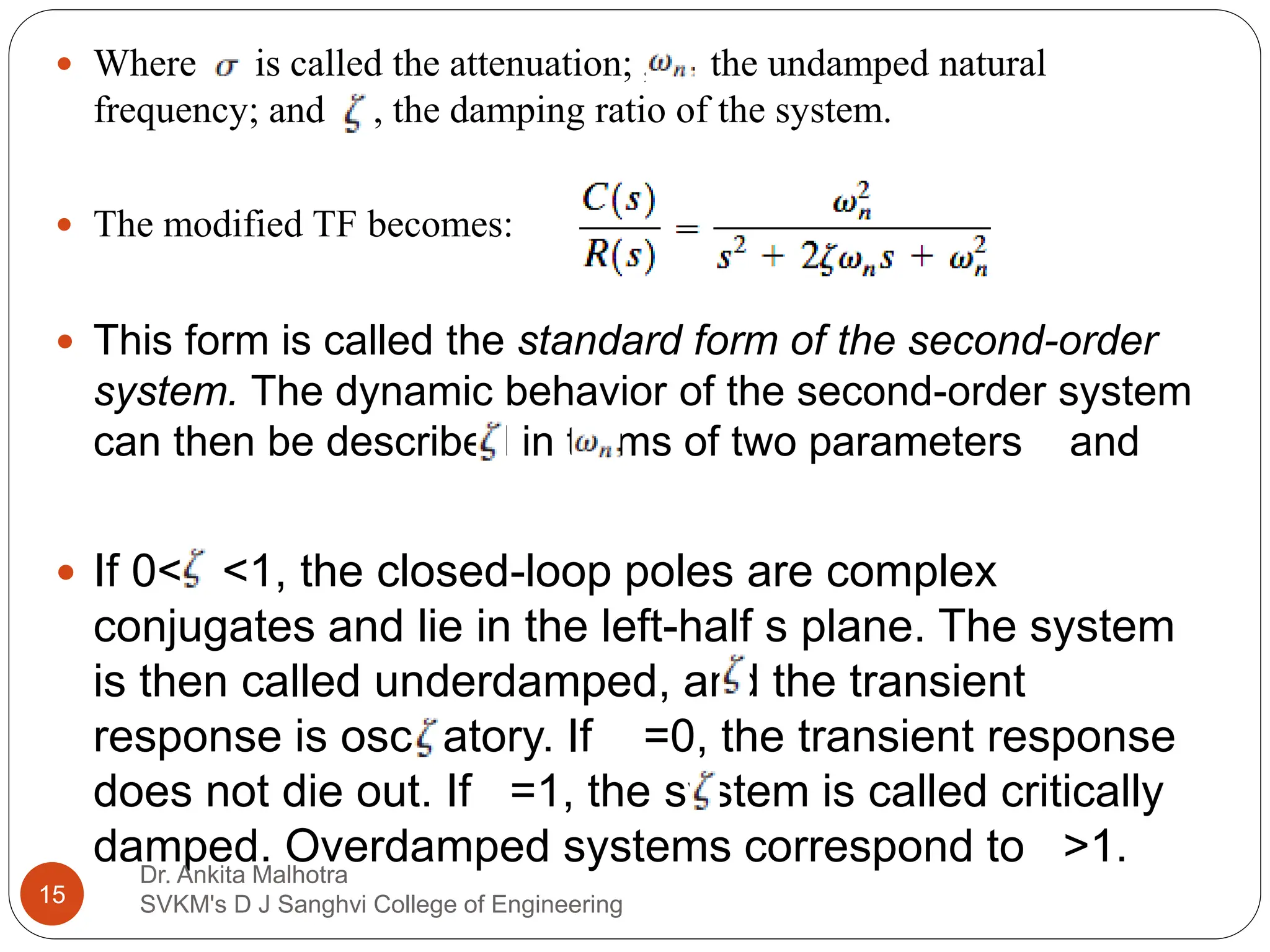
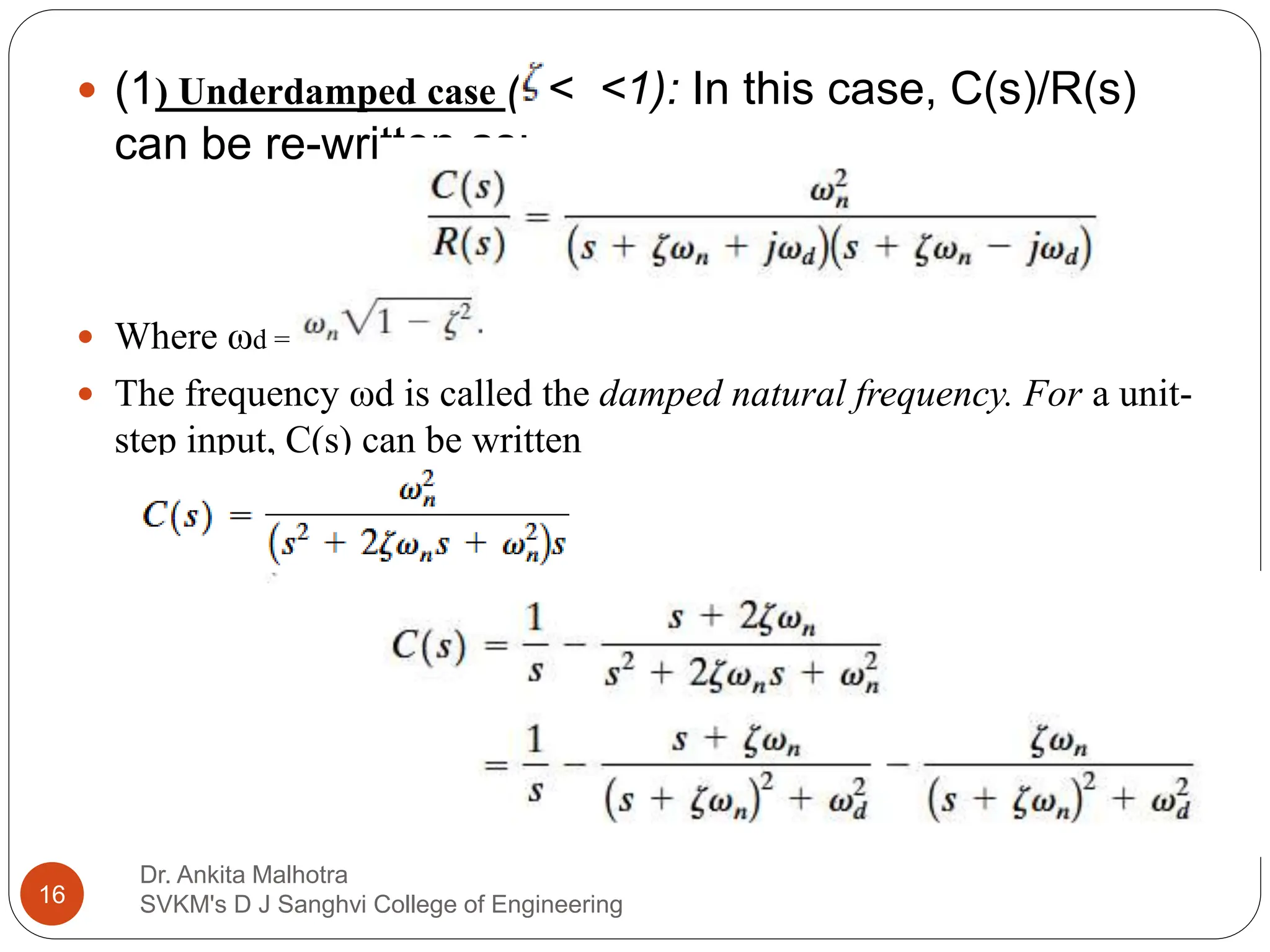
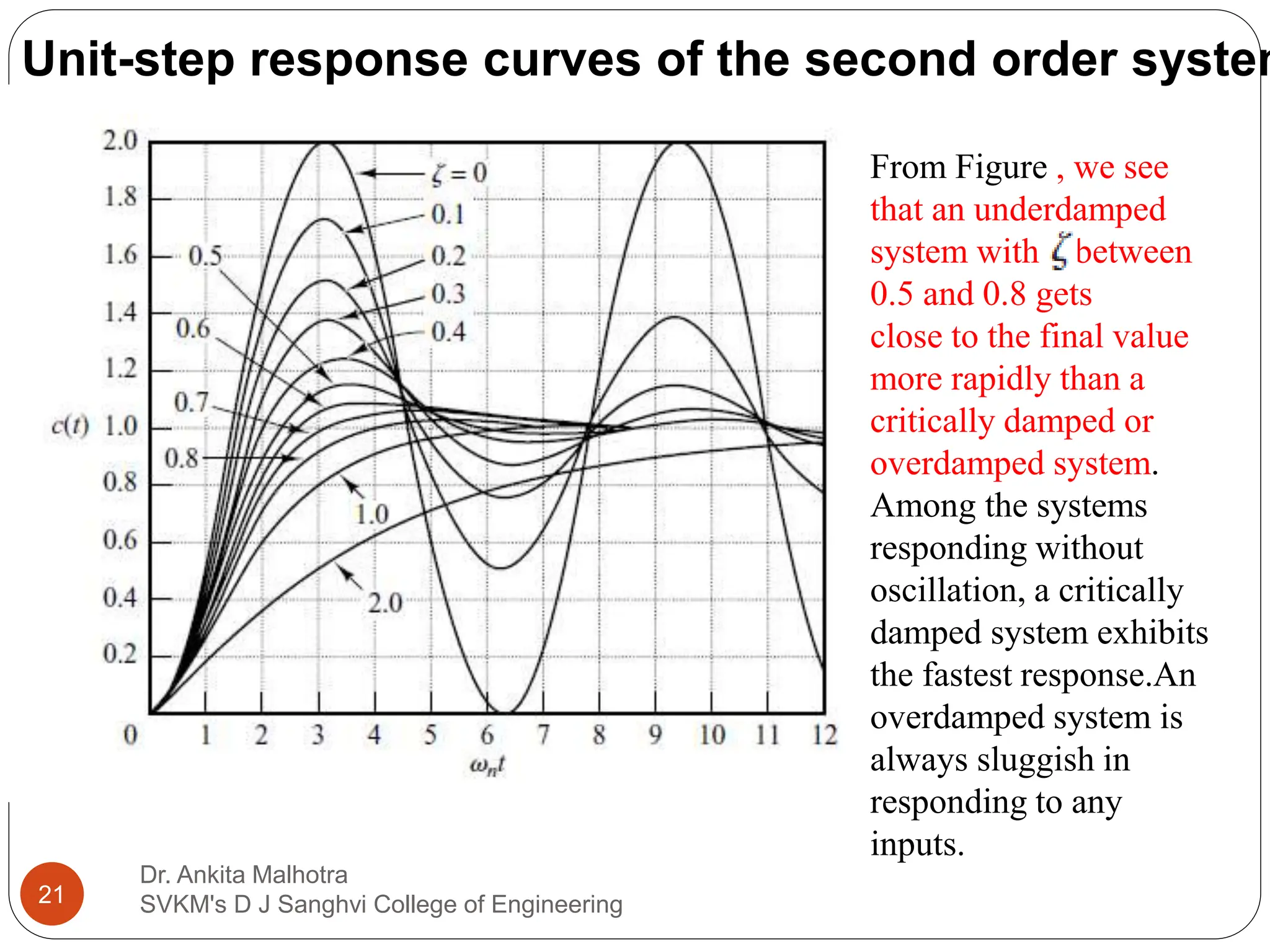
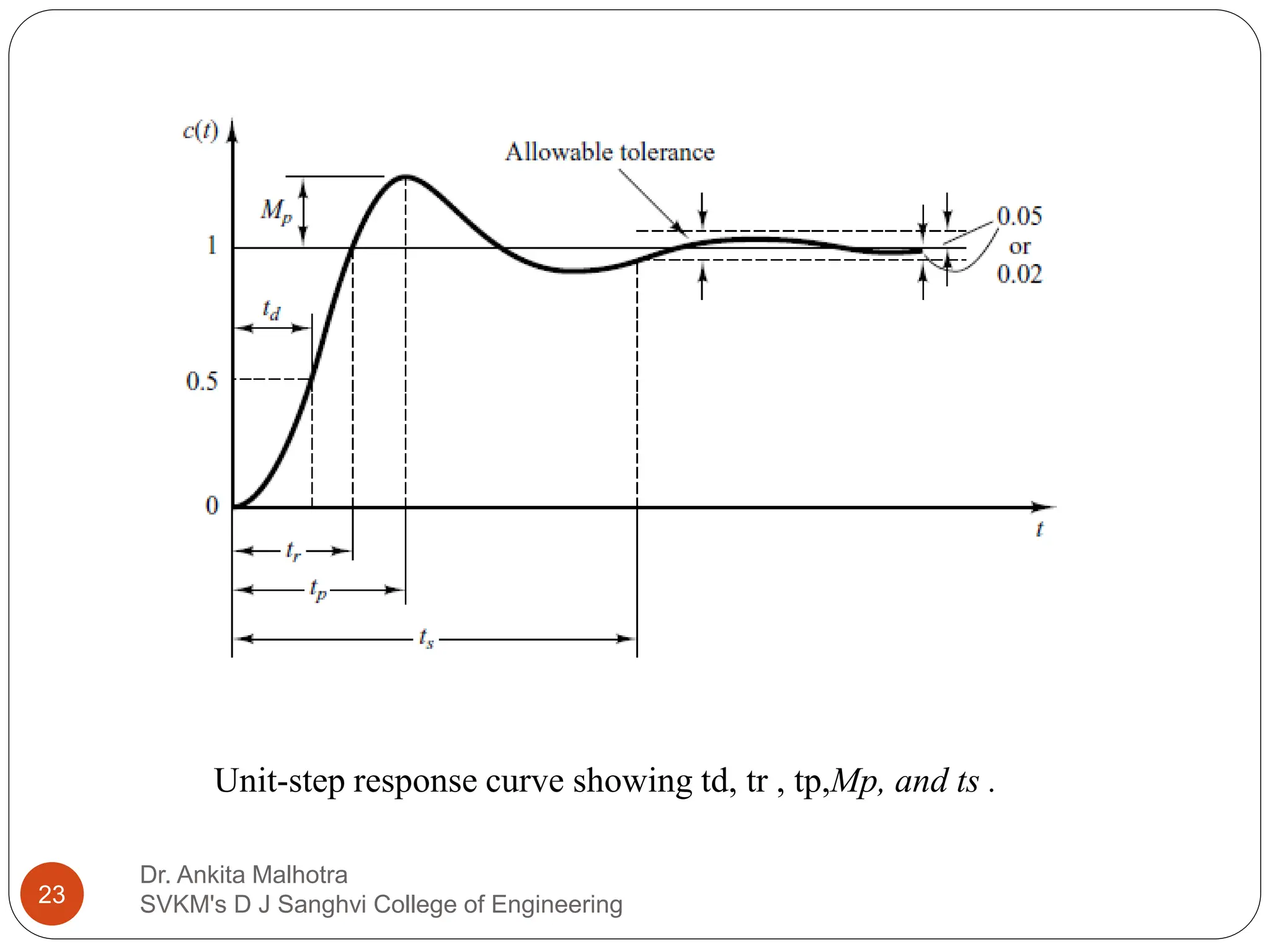
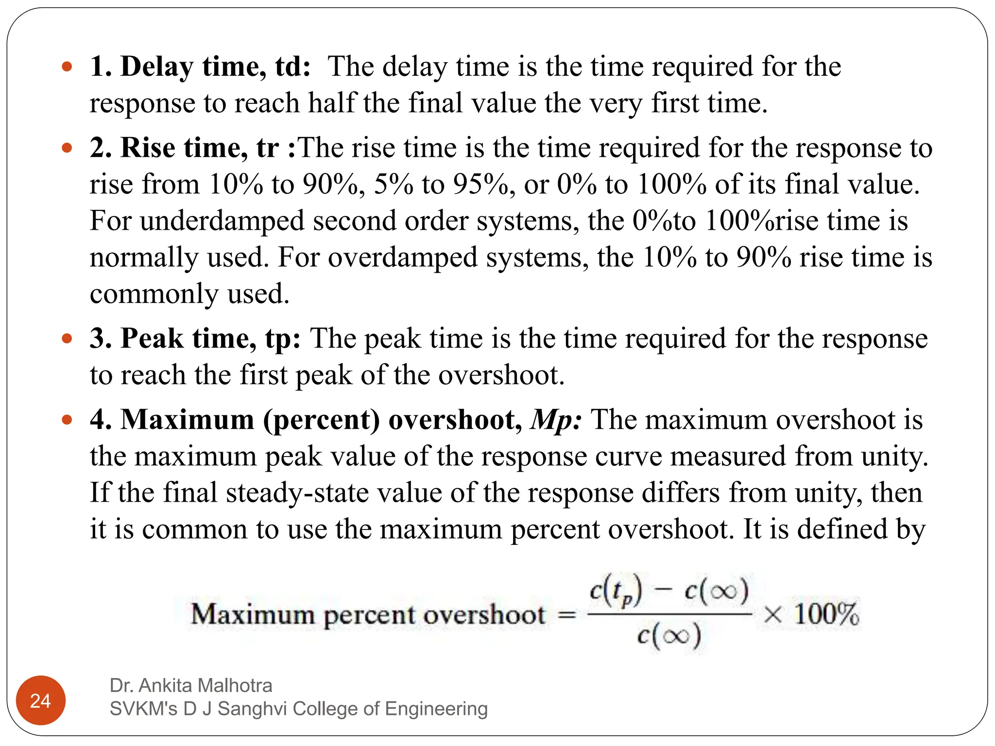
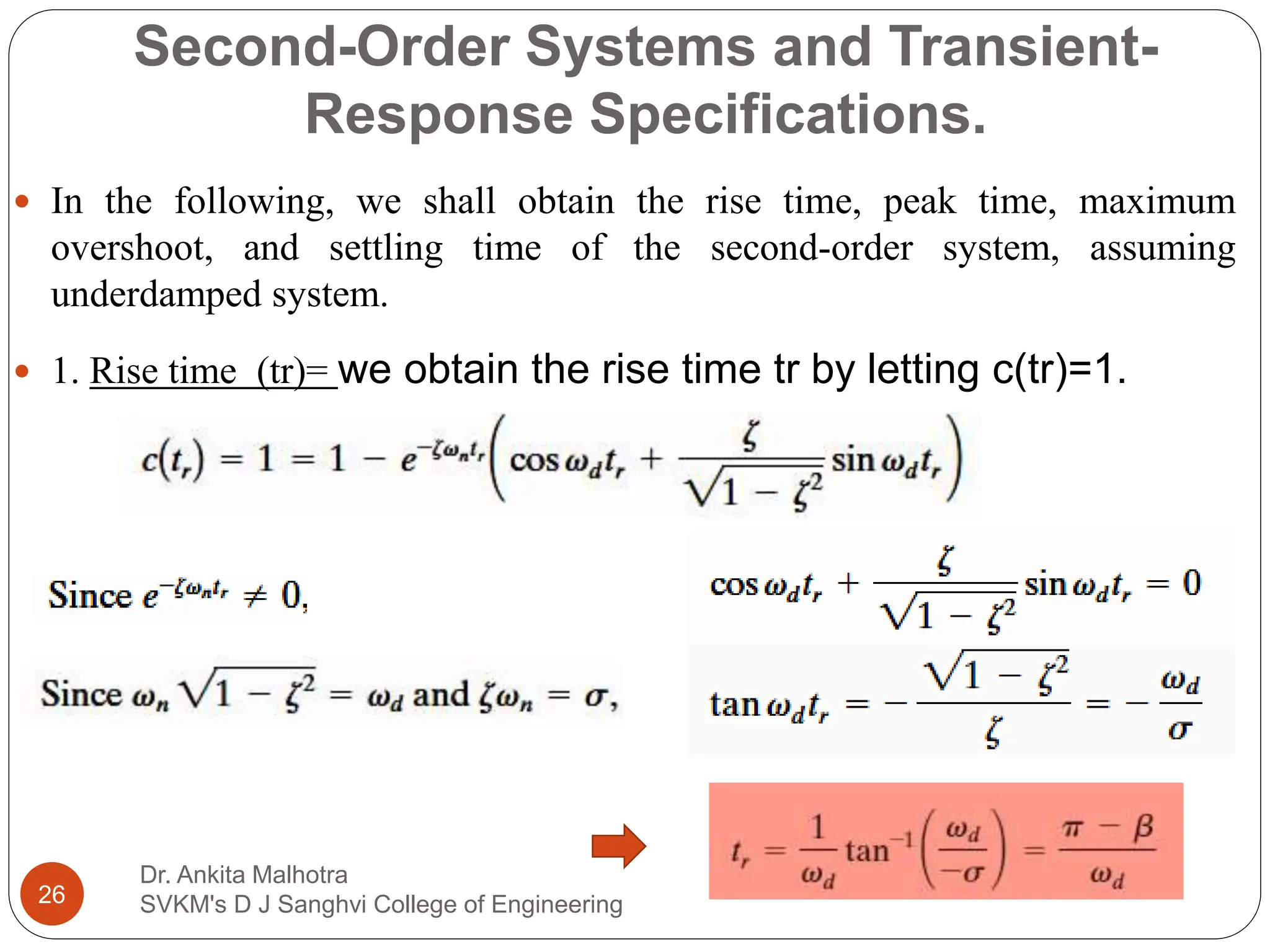
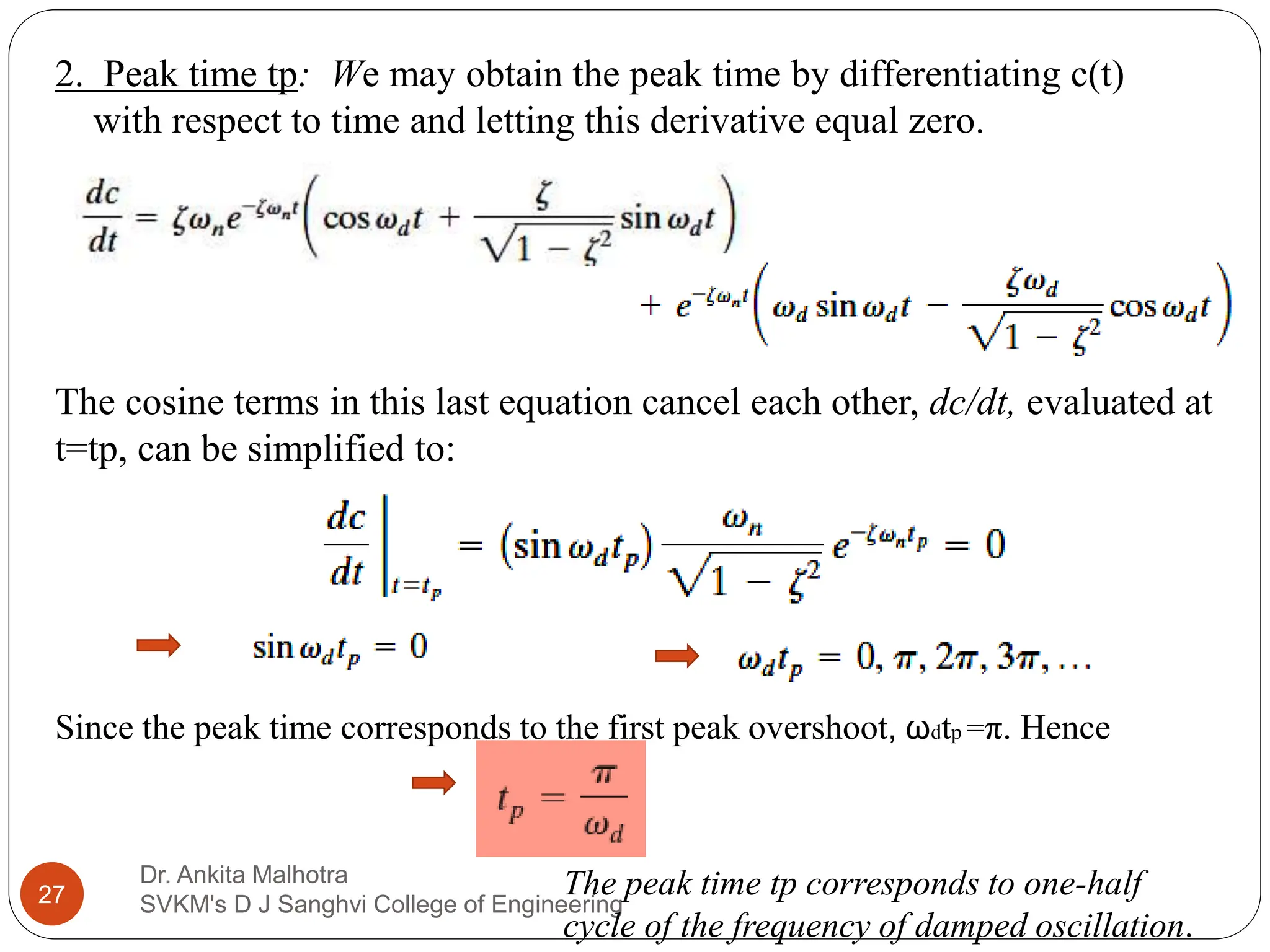
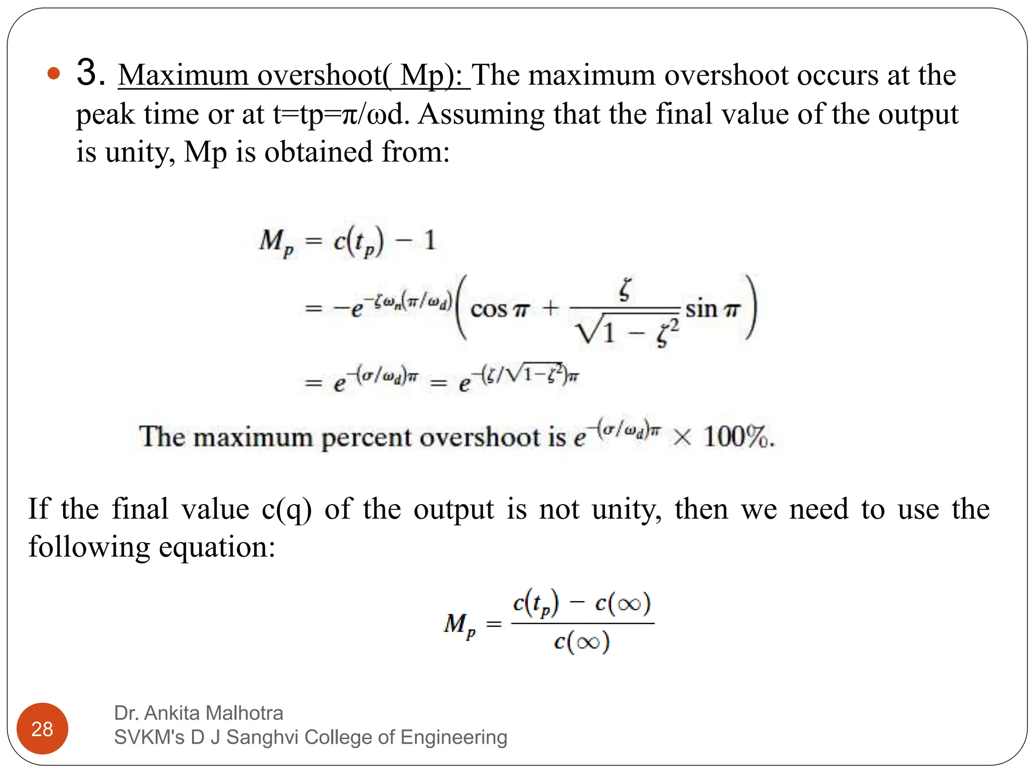
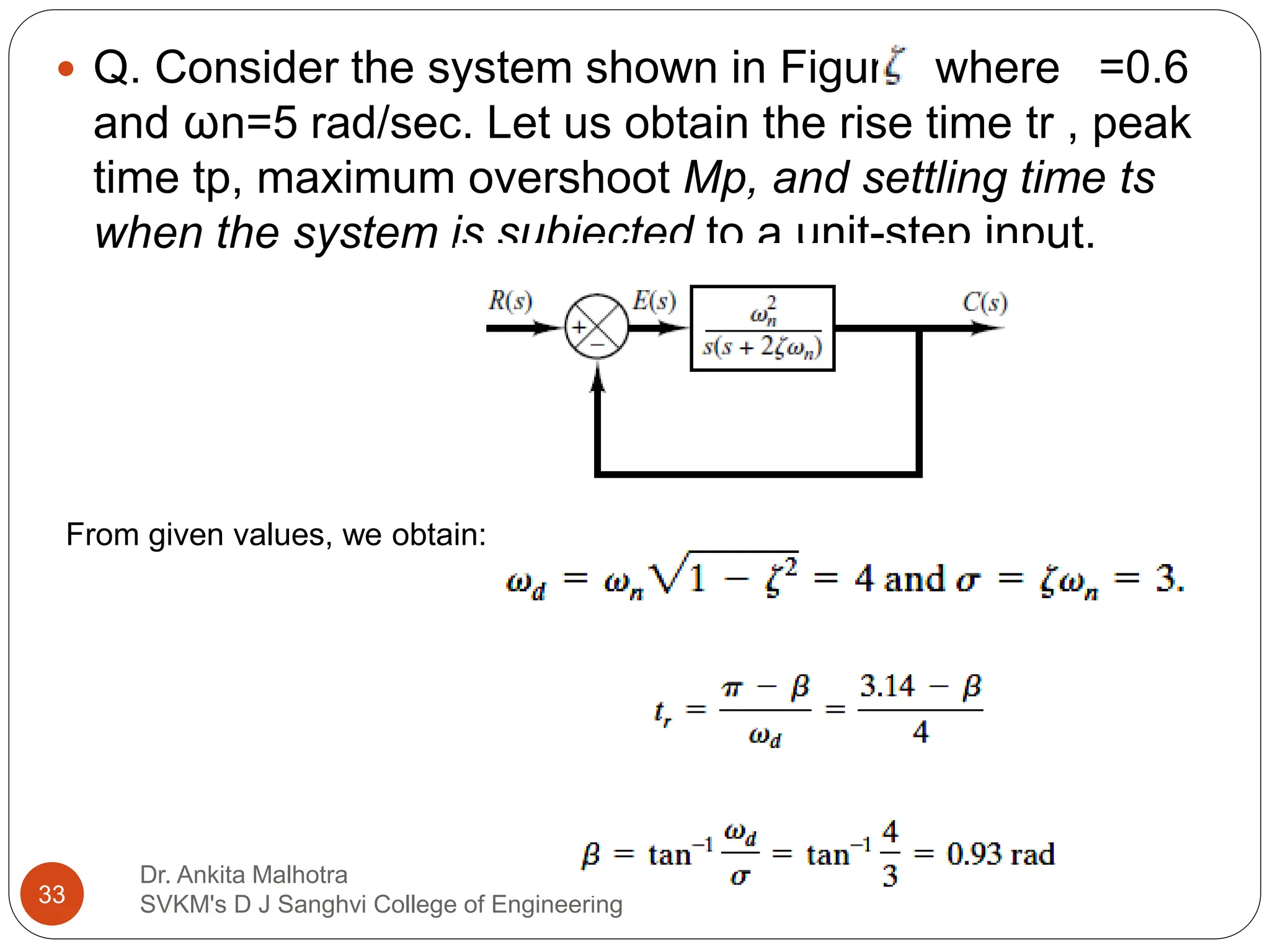
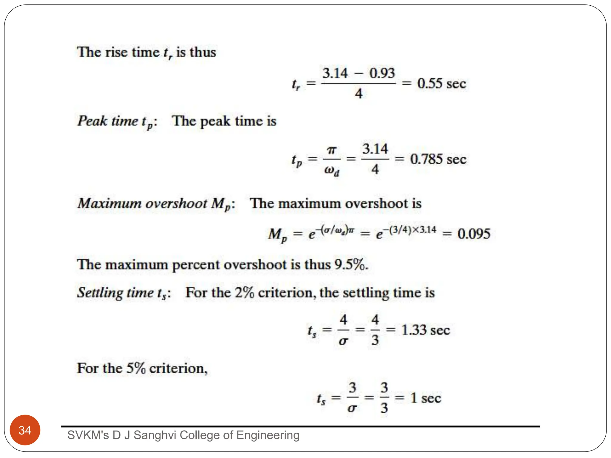
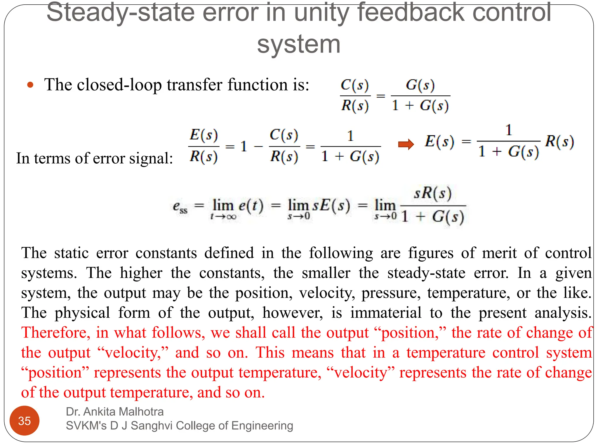
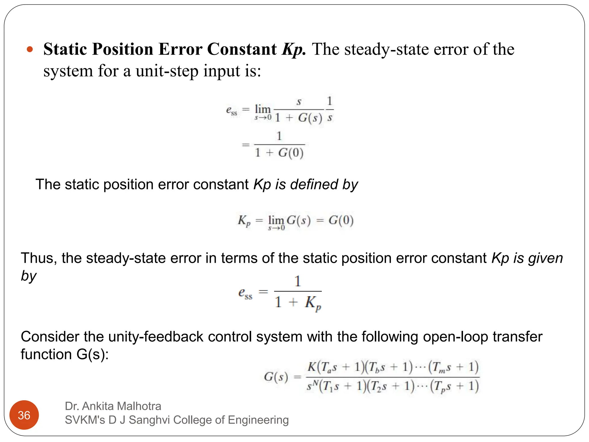
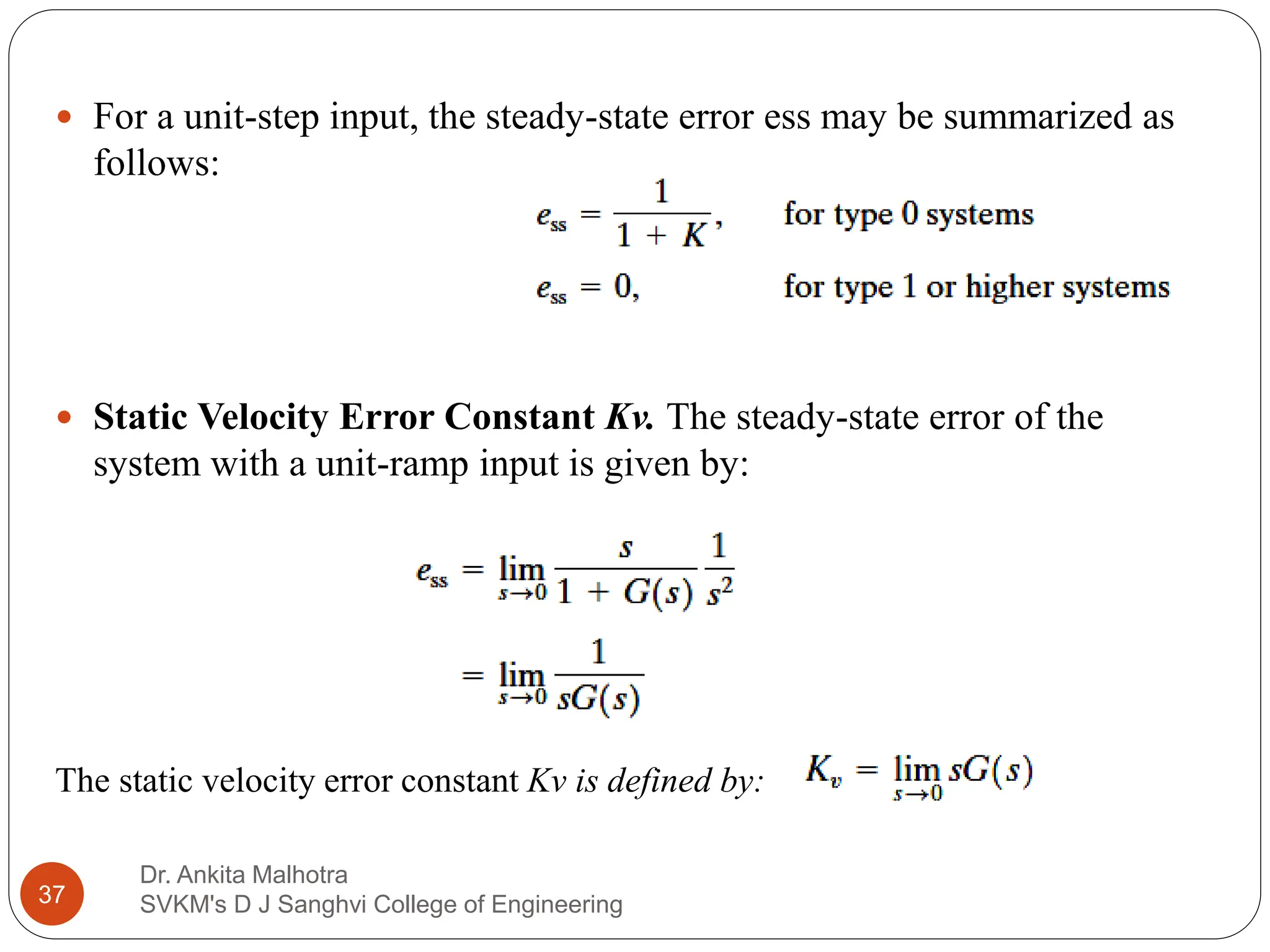
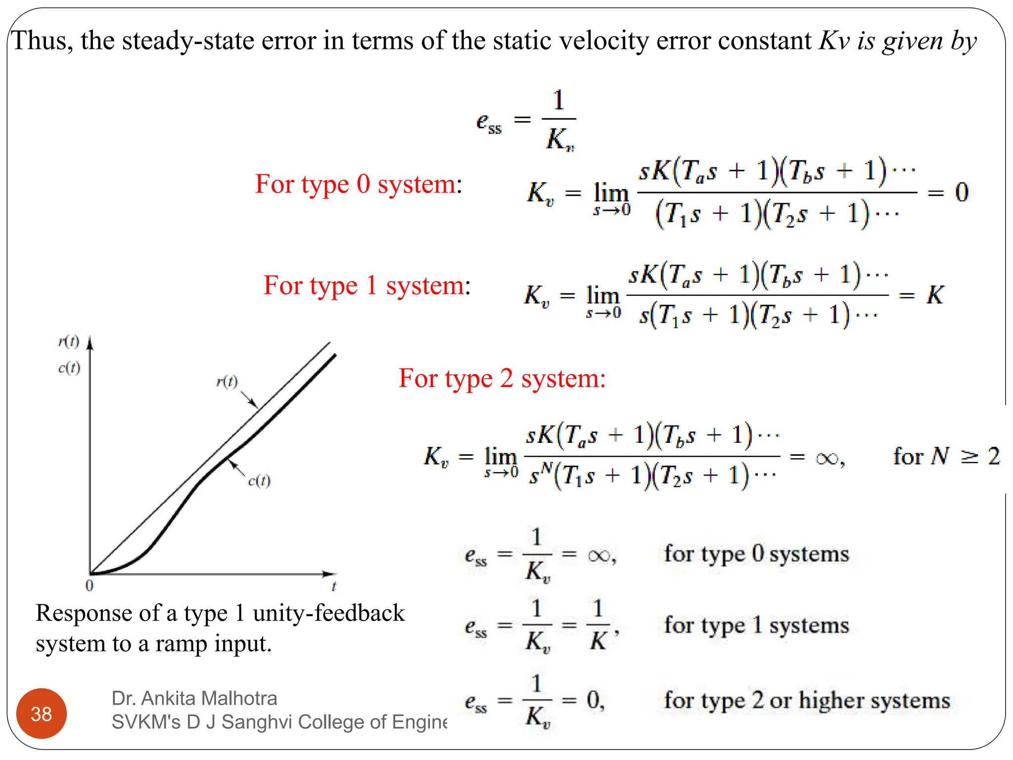
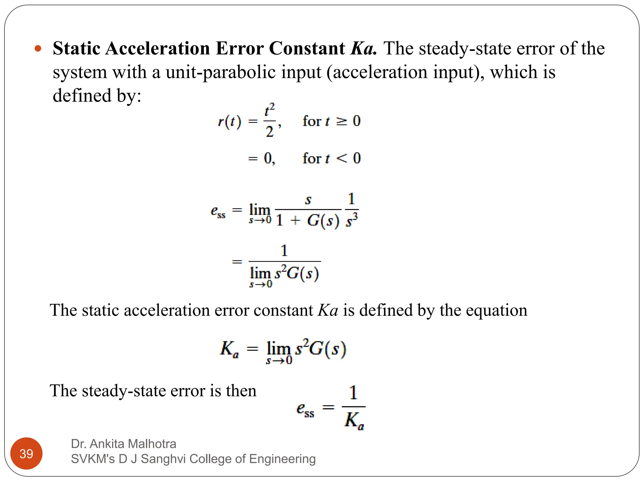
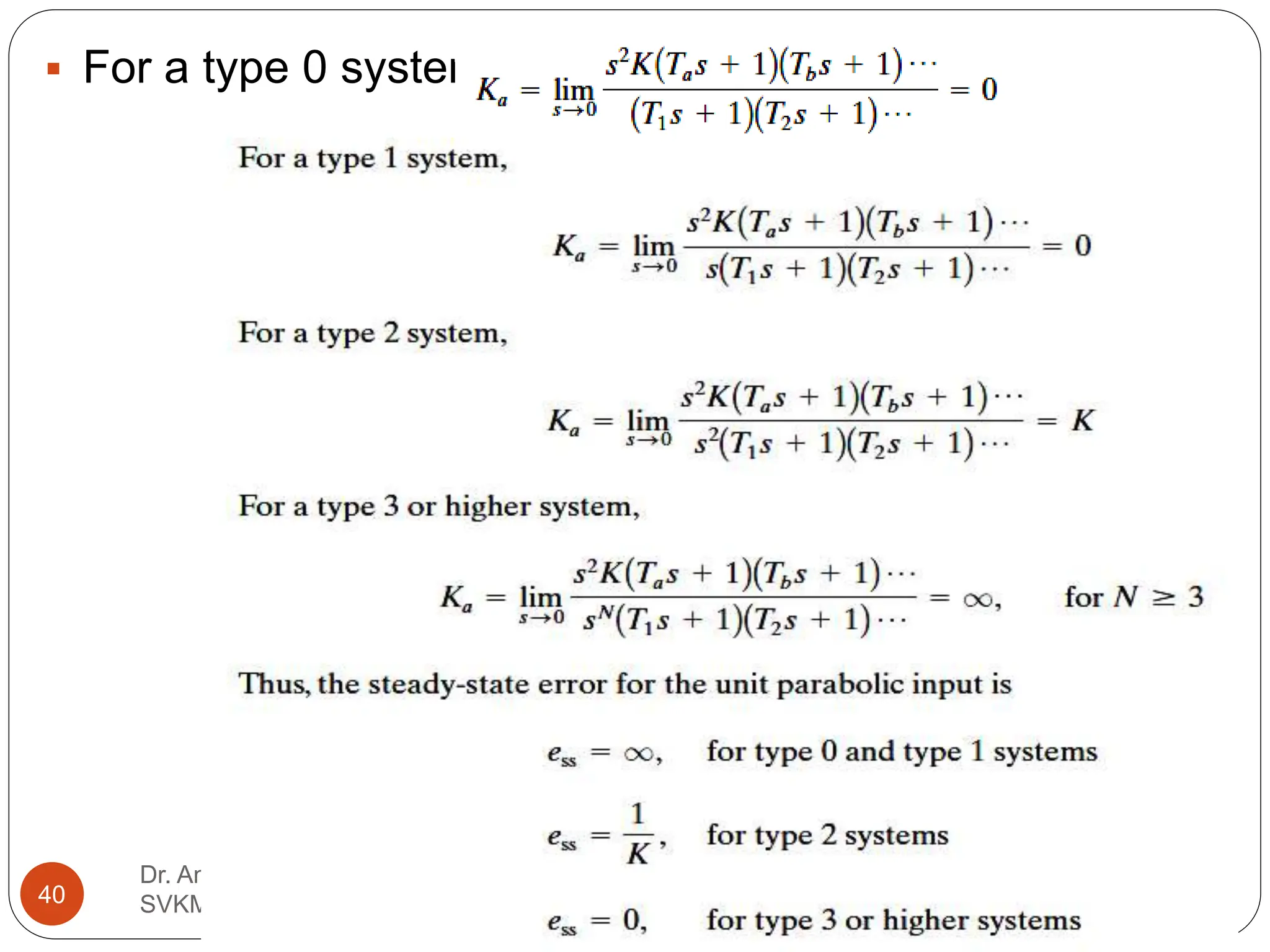
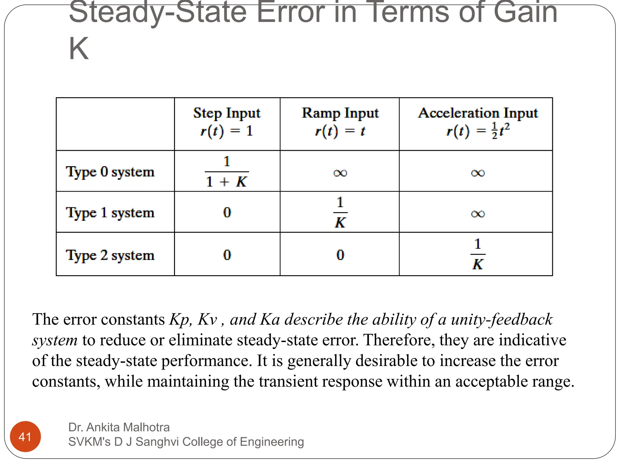
UNIT -4 (04 Hrs)
Response of control system
1
Dr. Ankita Malhotra
SVKM's D J Sanghvi College of Engineering
Standard Test Signals
In analyzing and designing control systems, we must have a basis of
comparison of performance of various control systems. This basis
may be set up by specifying particular test input signals and by
comparing the responses of various systems to these input signals.
The commonly used test input signals are:
 step functions,
 ramp functions,
 impulse functions,
 sinusoidal functions,
 and white noise
2
Dr. Ankita Malhotra
SVKM's D J Sanghvi College of Engineering
 Which of these typical input signals to use for analyzing system
characteristics may be determined by the form of the input that the
system will be subjected to most frequently under normal operation.
If the inputs to a control system are gradually changing functions of
time, then a ramp function of time may be a good test signal.
Similarly, if a system is subjected to sudden disturbances, a step
function of time may be a good test signal.
3
Dr. Ankita Malhotra
SVKM's D J Sanghvi College of Engineering
Transient Response and Steady-
State Response
The time response of a control system consists of
two parts: the transient response and the steady-
state response. By transient response, we mean
that which goes from the initial state to the final
state. By steady-state response, we mean the
manner in which the system output behaves as ‘t’
approaches infinity.
c(t) = ctr(t) + css(t)
4
Dr. Ankita Malhotra
SVKM's D J Sanghvi College of Engineering
FIRST ORDER SYSTEMS
 The input-output relationship is given by:
 C(s)/R(s) =1/(Ts + 1)
 In the following, we shall analyze the system
responses to such inputs as the unit-step, unit-
ramp, and unit-impulse functions. The initial
conditions are assumed to be zero.
First order systems
5
Dr. Ankita Malhotra
SVKM's D J Sanghvi College of Engineering
Unit-Step Response of First-Order
Systems
 Since the Laplace transform of the unit-step function is
1/s, substituting R(s)=1/s , we obtain:
C(s) =1/(Ts + 1)s
Expanding into partial fractions:
Taking the inverse Laplace transform:
 Equation states that initially the output c(t) is zero and
finally it becomes unity. One important characteristic of
such an exponential response curve c(t) is that at t=T the
value of c(t) is 0.632, or the response c(t) has reached
63.2% of its total change. This may be easily seen by
substituting t=T in c(t).That is,
c(T) = 1 - e-1 = 0.632
6
Dr. Ankita Malhotra
SVKM's D J Sanghvi College of Engineering
 Note that the smaller the time constant T, the faster the system response.
Another important characteristic of the exponential response curve is that the
slope of the tangent line at t=0 is 1/T, since
 The output would reach the final value at t=T if it maintained its initial speed
of response. In two time constants, the response reaches 86.5%of the final
value. At t=3T, 4T, and 5T, the response reaches 95%, 98.2%, and 99.3%,
respectively, of the final value.
7
Dr. Ankita Malhotra
SVKM's D J Sanghvi College of Engineering
Unit-Ramp Response of First-Order
Systems.
Since the Laplace transform of the unit-ramp function is
1/s2, we obtain the output of the system as:
Taking inverse laplace transform:
Error signal is given as:
8
Dr. Ankita Malhotra
SVKM's D J Sanghvi College of Engineering
As t approaches infinity, e–t/T approaches zero, and thus the error signal
e(t) approaches T.
The smaller the time constant T, the smaller the steady-state error in
following the ramp input.
9
Dr. Ankita Malhotra
SVKM's D J Sanghvi College of Engineering
Unit-Impulse Response of First-Order Systems.
 For the unit-impulse input, R(s)=1, the output of
the system can be given by:
 Tking inverse laplace transform:
10
Dr. Ankita Malhotra
SVKM's D J Sanghvi College of Engineering
Comparing the system responses to these three inputs clearly indicates that
the response to the derivative of an input signal can be obtained by
differentiating the response of the system to the original signal. It can also be
seen that the response to the integral of the original signal can be obtained by
integrating the response of the system to the original signal and by
determining the integration constant from the zero-output initial condition.
This is a property of linear time-invariant systems. Linear time-varying
systems and nonlinear systems do not possess this property.
11
Dr. Ankita Malhotra
SVKM's D J Sanghvi College of Engineering
Second Order Systems
 Consider the servo system consisting of a proportional controller and
load elements (inertia and viscous-friction elements).Suppose that we
wish to control the output position c in accordance with the input
position r.
The equation for the load elements is
where T is the torque produced by the proportional controller whose
gain is K. By taking Laplace transforms of both sides of this last
equation, assuming the zero initial conditions, we obtain:
12
Dr. Ankita Malhotra
SVKM's D J Sanghvi College of Engineering
Such a system where the closed-loop transfer function possesses two
poles is called a second-order system.
Block diagram of given second order system
13
Dr. Ankita Malhotra
SVKM's D J Sanghvi College of Engineering
Modified TF, considering gain K in the forward path
Step Response of Second-Order
System
 The closed-loop transfer function of the system is:
 which can be rewritten as
 The closed-loop poles are complex conjugates if B2-4JK<0 and
they are real if B2-4JK > 0.
 In the transient-response analysis, it is convenient to write
14
Dr. Ankita Malhotra
SVKM's D J Sanghvi College of Engineering
 Where is called the attenuation; , the undamped natural
frequency; and , the damping ratio of the system.
 The modified TF becomes:
 This form is called the standard form of the second-order
system. The dynamic behavior of the second-order system
can then be described in terms of two parameters and
 If 0< <1, the closed-loop poles are complex
conjugates and lie in the left-half s plane. The system
is then called underdamped, and the transient
response is oscillatory. If =0, the transient response
does not die out. If =1, the system is called critically
damped. Overdamped systems correspond to >1.
15
Dr. Ankita Malhotra
SVKM's D J Sanghvi College of Engineering
Dr. Ankita Malhotra
SVKM's D J Sanghvi College of Engineering
16
 (1) Underdamped case (0< <1): In this case, C(s)/R(s)
can be re-written as:
 Where ωd =
 The frequency ωd is called the damped natural frequency. For a unit-
step input, C(s) can be written
Dr. Ankita Malhotra
SVKM's D J Sanghvi College of Engineering
17
It can be seen that the frequency of transient oscillation is the damped
natural frequency ωd and thus varies with the damping ratio .
Dr. Ankita Malhotra
SVKM's D J Sanghvi College of Engineering
18
 The error signal for this system is the difference between the input and
output and is
 This error signal exhibits a damped sinusoidal oscillation. At steady
state, or at t=∞,no error exists between the input and output.
 If the damping ratio is equal to zero, the response becomes
undamped and oscillations continue indefinitely. The response c(t) for
the zero damping case may be obtained by substituting =0 in the
expression of c(t).
Undamped natural frequency of the system
Dr. Ankita Malhotra
SVKM's D J Sanghvi College of Engineering
19
(2) Critically damped case ( =1): If the two poles of C(s)/R(s) are
equal, the system is said to be a critically damped one.
 For approaching unity in the expression of c(t) and by using the
following limit:
(3) Overdamped case ( >1 ):
 In this case, the two poles of C(s)/R(s) are negative real and unequal.
For a unit-step input, R(s)=1/s and C(s) can be written
Dr. Ankita Malhotra
SVKM's D J Sanghvi College of Engineering
20
 Taking inverse Laplace transform
Thus, the response c(t) includes two decaying exponential terms.
Suppose –s2 is located very much closer to the jω axis than –s1 (which
means |s2| << |s1| ), then for an approximate solution we may neglect –
s1. This is permissible because the effect of –s1 on the response
is much smaller than that of –s2.
Unit-step response curves of the second order system
Dr. Ankita Malhotra
SVKM's D J Sanghvi College of Engineering
21
From Figure , we see
that an underdamped
system with between
0.5 and 0.8 gets
close to the final value
more rapidly than a
critically damped or
overdamped system.
Among the systems
responding without
oscillation, a critically
damped system exhibits
the fastest response.An
overdamped system is
always sluggish in
responding to any
inputs.
Definitions of Transient-Response
Specifications
Dr. Ankita Malhotra
SVKM's D J Sanghvi College of Engineering
22
The transient response of a practical control system often exhibits
damped oscillations before reaching steady state. In specifying the
transient-response characteristics of a control system to a unit-step
input, it is common to specify the following:
 1. Delay time, td
 2. Rise time, tr
 3. Peak time, tp
 4. Maximum overshoot,Mp
 5. Settling time, ts
Dr. Ankita Malhotra
SVKM's D J Sanghvi College of Engineering
23
Unit-step response curve showing td, tr , tp,Mp, and ts .
Dr. Ankita Malhotra
SVKM's D J Sanghvi College of Engineering
24
 1. Delay time, td: The delay time is the time required for the
response to reach half the final value the very first time.
 2. Rise time, tr :The rise time is the time required for the response to
rise from 10% to 90%, 5% to 95%, or 0% to 100% of its final value.
For underdamped second order systems, the 0%to 100%rise time is
normally used. For overdamped systems, the 10% to 90% rise time is
commonly used.
 3. Peak time, tp: The peak time is the time required for the response
to reach the first peak of the overshoot.
 4. Maximum (percent) overshoot, Mp: The maximum overshoot is
the maximum peak value of the response curve measured from unity.
If the final steady-state value of the response differs from unity, then
it is common to use the maximum percent overshoot. It is defined by
Dr. Ankita Malhotra
SVKM's D J Sanghvi College of Engineering
25
The amount of the maximum (percent) overshoot directly indicates
the relative stability of the system.
 5. Settling time, ts : The settling time is the time required for the
response curve to reach and stay within a range about the final
value of size specified by absolute percentage of the final value
(usually 2% or 5%). The settling time is related to the largest time
constant of the control system.
Second-Order Systems and Transient-
Response Specifications.
Dr. Ankita Malhotra
SVKM's D J Sanghvi College of Engineering
26
 In the following, we shall obtain the rise time, peak time, maximum
overshoot, and settling time of the second-order system, assuming
underdamped system.
 1. Rise time (tr)= we obtain the rise time tr by letting c(tr)=1.
Dr. Ankita Malhotra
SVKM's D J Sanghvi College of Engineering
27
2. Peak time tp: We may obtain the peak time by differentiating c(t)
with respect to time and letting this derivative equal zero.
The cosine terms in this last equation cancel each other, dc/dt, evaluated at
t=tp, can be simplified to:
Since the peak time corresponds to the first peak overshoot, ωdtp =π. Hence
The peak time tp corresponds to one-half
cycle of the frequency of damped oscillation.
Dr. Ankita Malhotra
SVKM's D J Sanghvi College of Engineering
28
 3. Maximum overshoot( Mp): The maximum overshoot occurs at the
peak time or at t=tp=π/ωd. Assuming that the final value of the output
is unity, Mp is obtained from:
If the final value c(q) of the output is not unity, then we need to use the
following equation:
Dr. Ankita Malhotra
SVKM's D J Sanghvi College of Engineering
29
 Settling time (ts) : For an underdamped second-order system, the
transient response is given as:
Dr. Ankita Malhotra
SVKM's D J Sanghvi College of Engineering
30
 The speed of decay of the transient response depends on the value of
the time constant . The settling time corresponding to a ; 2% or
;5% tolerance band may be measured in terms of the time constant
T= from the curves of Figure 5–7 for different values of .The
results are shown in Figure 5–11. For 0< <0.9, if the 2% criterion is
used, ts is approximately four times the time constant of the system.
If the 5% criterion is used, then ts is approximately three times the
time constant. Note that the settling time reaches a minimum value
around =0.76 (for the 2% criterion) or =0.68 (for the 5%
criterion) and then increases almost linearly for large values of .
Practice problems
Dr. Ankita Malhotra
SVKM's D J Sanghvi College of Engineering
31
 Q.When the system shown in Figure (a) is subjected to a unit-step input, the
system output responds as shown in Figure (b). Determine the values of K
and T from the response curve.
Dr. Ankita Malhotra
SVKM's D J Sanghvi College of Engineering
32
 The maximum overshoot of 25.4% corresponds to
=0.4. From the response curve we have:
Dr. Ankita Malhotra
SVKM's D J Sanghvi College of Engineering
33
 Q. Consider the system shown in Figure, where =0.6
and ωn=5 rad/sec. Let us obtain the rise time tr , peak
time tp, maximum overshoot Mp, and settling time ts
when the system is subjected to a unit-step input.
From given values, we obtain:
Dr. Ankita Malhotra
SVKM's D J Sanghvi College of Engineering
34
Steady-state error in unity feedback control
system
Dr. Ankita Malhotra
SVKM's D J Sanghvi College of Engineering
35
 The closed-loop transfer function is:
The static error constants defined in the following are figures of merit of control
systems. The higher the constants, the smaller the steady-state error. In a given
system, the output may be the position, velocity, pressure, temperature, or the like.
The physical form of the output, however, is immaterial to the present analysis.
Therefore, in what follows, we shall call the output “position,” the rate of change of
the output “velocity,” and so on. This means that in a temperature control system
“position” represents the output temperature, “velocity” represents the rate of change
of the output temperature, and so on.
In terms of error signal:
Dr. Ankita Malhotra
SVKM's D J Sanghvi College of Engineering
36
 Static Position Error Constant Kp. The steady-state error of the
system for a unit-step input is:
The static position error constant Kp is defined by
Thus, the steady-state error in terms of the static position error constant Kp is given
by
Consider the unity-feedback control system with the following open-loop transfer
function G(s):
Dr. Ankita Malhotra
SVKM's D J Sanghvi College of Engineering
37
 For a unit-step input, the steady-state error ess may be summarized as
follows:
 Static Velocity Error Constant Kv. The steady-state error of the
system with a unit-ramp input is given by:
The static velocity error constant Kv is defined by:
Dr. Ankita Malhotra
SVKM's D J Sanghvi College of Engineering
38
Thus, the steady-state error in terms of the static velocity error constant Kv is given by
Response of a type 1 unity-feedback
system to a ramp input.
For type 0 system:
For type 1 system:
For type 2 system:
Dr. Ankita Malhotra
SVKM's D J Sanghvi College of Engineering
39
 Static Acceleration Error Constant Ka. The steady-state error of the
system with a unit-parabolic input (acceleration input), which is
defined by:
The static acceleration error constant Ka is defined by the equation
The steady-state error is then
Dr. Ankita Malhotra
SVKM's D J Sanghvi College of Engineering
40
 For a type 0 system,
Steady-State Error in Terms of Gain
K
Dr. Ankita Malhotra
SVKM's D J Sanghvi College of Engineering
41
The error constants Kp, Kv , and Ka describe the ability of a unity-feedback
system to reduce or eliminate steady-state error. Therefore, they are indicative
of the steady-state performance. It is generally desirable to increase the error
constants, while maintaining the transient response within an acceptable range.

Response of control systems in time domain

  • 1.
    UNIT -4 (04Hrs) Response of control system 1 Dr. Ankita Malhotra SVKM's D J Sanghvi College of Engineering
  • 2.
    Standard Test Signals Inanalyzing and designing control systems, we must have a basis of comparison of performance of various control systems. This basis may be set up by specifying particular test input signals and by comparing the responses of various systems to these input signals. The commonly used test input signals are:  step functions,  ramp functions,  impulse functions,  sinusoidal functions,  and white noise 2 Dr. Ankita Malhotra SVKM's D J Sanghvi College of Engineering
  • 3.
     Which ofthese typical input signals to use for analyzing system characteristics may be determined by the form of the input that the system will be subjected to most frequently under normal operation. If the inputs to a control system are gradually changing functions of time, then a ramp function of time may be a good test signal. Similarly, if a system is subjected to sudden disturbances, a step function of time may be a good test signal. 3 Dr. Ankita Malhotra SVKM's D J Sanghvi College of Engineering
  • 4.
    Transient Response andSteady- State Response The time response of a control system consists of two parts: the transient response and the steady- state response. By transient response, we mean that which goes from the initial state to the final state. By steady-state response, we mean the manner in which the system output behaves as ‘t’ approaches infinity. c(t) = ctr(t) + css(t) 4 Dr. Ankita Malhotra SVKM's D J Sanghvi College of Engineering
  • 5.
    FIRST ORDER SYSTEMS The input-output relationship is given by:  C(s)/R(s) =1/(Ts + 1)  In the following, we shall analyze the system responses to such inputs as the unit-step, unit- ramp, and unit-impulse functions. The initial conditions are assumed to be zero. First order systems 5 Dr. Ankita Malhotra SVKM's D J Sanghvi College of Engineering
  • 6.
    Unit-Step Response ofFirst-Order Systems  Since the Laplace transform of the unit-step function is 1/s, substituting R(s)=1/s , we obtain: C(s) =1/(Ts + 1)s Expanding into partial fractions: Taking the inverse Laplace transform:  Equation states that initially the output c(t) is zero and finally it becomes unity. One important characteristic of such an exponential response curve c(t) is that at t=T the value of c(t) is 0.632, or the response c(t) has reached 63.2% of its total change. This may be easily seen by substituting t=T in c(t).That is, c(T) = 1 - e-1 = 0.632 6 Dr. Ankita Malhotra SVKM's D J Sanghvi College of Engineering
  • 7.
     Note thatthe smaller the time constant T, the faster the system response. Another important characteristic of the exponential response curve is that the slope of the tangent line at t=0 is 1/T, since  The output would reach the final value at t=T if it maintained its initial speed of response. In two time constants, the response reaches 86.5%of the final value. At t=3T, 4T, and 5T, the response reaches 95%, 98.2%, and 99.3%, respectively, of the final value. 7 Dr. Ankita Malhotra SVKM's D J Sanghvi College of Engineering
  • 8.
    Unit-Ramp Response ofFirst-Order Systems. Since the Laplace transform of the unit-ramp function is 1/s2, we obtain the output of the system as: Taking inverse laplace transform: Error signal is given as: 8 Dr. Ankita Malhotra SVKM's D J Sanghvi College of Engineering
  • 9.
    As t approachesinfinity, e–t/T approaches zero, and thus the error signal e(t) approaches T. The smaller the time constant T, the smaller the steady-state error in following the ramp input. 9 Dr. Ankita Malhotra SVKM's D J Sanghvi College of Engineering
  • 10.
    Unit-Impulse Response ofFirst-Order Systems.  For the unit-impulse input, R(s)=1, the output of the system can be given by:  Tking inverse laplace transform: 10 Dr. Ankita Malhotra SVKM's D J Sanghvi College of Engineering
  • 11.
    Comparing the systemresponses to these three inputs clearly indicates that the response to the derivative of an input signal can be obtained by differentiating the response of the system to the original signal. It can also be seen that the response to the integral of the original signal can be obtained by integrating the response of the system to the original signal and by determining the integration constant from the zero-output initial condition. This is a property of linear time-invariant systems. Linear time-varying systems and nonlinear systems do not possess this property. 11 Dr. Ankita Malhotra SVKM's D J Sanghvi College of Engineering
  • 12.
    Second Order Systems Consider the servo system consisting of a proportional controller and load elements (inertia and viscous-friction elements).Suppose that we wish to control the output position c in accordance with the input position r. The equation for the load elements is where T is the torque produced by the proportional controller whose gain is K. By taking Laplace transforms of both sides of this last equation, assuming the zero initial conditions, we obtain: 12 Dr. Ankita Malhotra SVKM's D J Sanghvi College of Engineering
  • 13.
    Such a systemwhere the closed-loop transfer function possesses two poles is called a second-order system. Block diagram of given second order system 13 Dr. Ankita Malhotra SVKM's D J Sanghvi College of Engineering Modified TF, considering gain K in the forward path
  • 14.
    Step Response ofSecond-Order System  The closed-loop transfer function of the system is:  which can be rewritten as  The closed-loop poles are complex conjugates if B2-4JK<0 and they are real if B2-4JK > 0.  In the transient-response analysis, it is convenient to write 14 Dr. Ankita Malhotra SVKM's D J Sanghvi College of Engineering
  • 15.
     Where iscalled the attenuation; , the undamped natural frequency; and , the damping ratio of the system.  The modified TF becomes:  This form is called the standard form of the second-order system. The dynamic behavior of the second-order system can then be described in terms of two parameters and  If 0< <1, the closed-loop poles are complex conjugates and lie in the left-half s plane. The system is then called underdamped, and the transient response is oscillatory. If =0, the transient response does not die out. If =1, the system is called critically damped. Overdamped systems correspond to >1. 15 Dr. Ankita Malhotra SVKM's D J Sanghvi College of Engineering
  • 16.
    Dr. Ankita Malhotra SVKM'sD J Sanghvi College of Engineering 16  (1) Underdamped case (0< <1): In this case, C(s)/R(s) can be re-written as:  Where ωd =  The frequency ωd is called the damped natural frequency. For a unit- step input, C(s) can be written
  • 17.
    Dr. Ankita Malhotra SVKM'sD J Sanghvi College of Engineering 17 It can be seen that the frequency of transient oscillation is the damped natural frequency ωd and thus varies with the damping ratio .
  • 18.
    Dr. Ankita Malhotra SVKM'sD J Sanghvi College of Engineering 18  The error signal for this system is the difference between the input and output and is  This error signal exhibits a damped sinusoidal oscillation. At steady state, or at t=∞,no error exists between the input and output.  If the damping ratio is equal to zero, the response becomes undamped and oscillations continue indefinitely. The response c(t) for the zero damping case may be obtained by substituting =0 in the expression of c(t). Undamped natural frequency of the system
  • 19.
    Dr. Ankita Malhotra SVKM'sD J Sanghvi College of Engineering 19 (2) Critically damped case ( =1): If the two poles of C(s)/R(s) are equal, the system is said to be a critically damped one.  For approaching unity in the expression of c(t) and by using the following limit: (3) Overdamped case ( >1 ):  In this case, the two poles of C(s)/R(s) are negative real and unequal. For a unit-step input, R(s)=1/s and C(s) can be written
  • 20.
    Dr. Ankita Malhotra SVKM'sD J Sanghvi College of Engineering 20  Taking inverse Laplace transform Thus, the response c(t) includes two decaying exponential terms. Suppose –s2 is located very much closer to the jω axis than –s1 (which means |s2| << |s1| ), then for an approximate solution we may neglect – s1. This is permissible because the effect of –s1 on the response is much smaller than that of –s2.
  • 21.
    Unit-step response curvesof the second order system Dr. Ankita Malhotra SVKM's D J Sanghvi College of Engineering 21 From Figure , we see that an underdamped system with between 0.5 and 0.8 gets close to the final value more rapidly than a critically damped or overdamped system. Among the systems responding without oscillation, a critically damped system exhibits the fastest response.An overdamped system is always sluggish in responding to any inputs.
  • 22.
    Definitions of Transient-Response Specifications Dr.Ankita Malhotra SVKM's D J Sanghvi College of Engineering 22 The transient response of a practical control system often exhibits damped oscillations before reaching steady state. In specifying the transient-response characteristics of a control system to a unit-step input, it is common to specify the following:  1. Delay time, td  2. Rise time, tr  3. Peak time, tp  4. Maximum overshoot,Mp  5. Settling time, ts
  • 23.
    Dr. Ankita Malhotra SVKM'sD J Sanghvi College of Engineering 23 Unit-step response curve showing td, tr , tp,Mp, and ts .
  • 24.
    Dr. Ankita Malhotra SVKM'sD J Sanghvi College of Engineering 24  1. Delay time, td: The delay time is the time required for the response to reach half the final value the very first time.  2. Rise time, tr :The rise time is the time required for the response to rise from 10% to 90%, 5% to 95%, or 0% to 100% of its final value. For underdamped second order systems, the 0%to 100%rise time is normally used. For overdamped systems, the 10% to 90% rise time is commonly used.  3. Peak time, tp: The peak time is the time required for the response to reach the first peak of the overshoot.  4. Maximum (percent) overshoot, Mp: The maximum overshoot is the maximum peak value of the response curve measured from unity. If the final steady-state value of the response differs from unity, then it is common to use the maximum percent overshoot. It is defined by
  • 25.
    Dr. Ankita Malhotra SVKM'sD J Sanghvi College of Engineering 25 The amount of the maximum (percent) overshoot directly indicates the relative stability of the system.  5. Settling time, ts : The settling time is the time required for the response curve to reach and stay within a range about the final value of size specified by absolute percentage of the final value (usually 2% or 5%). The settling time is related to the largest time constant of the control system.
  • 26.
    Second-Order Systems andTransient- Response Specifications. Dr. Ankita Malhotra SVKM's D J Sanghvi College of Engineering 26  In the following, we shall obtain the rise time, peak time, maximum overshoot, and settling time of the second-order system, assuming underdamped system.  1. Rise time (tr)= we obtain the rise time tr by letting c(tr)=1.
  • 27.
    Dr. Ankita Malhotra SVKM'sD J Sanghvi College of Engineering 27 2. Peak time tp: We may obtain the peak time by differentiating c(t) with respect to time and letting this derivative equal zero. The cosine terms in this last equation cancel each other, dc/dt, evaluated at t=tp, can be simplified to: Since the peak time corresponds to the first peak overshoot, ωdtp =π. Hence The peak time tp corresponds to one-half cycle of the frequency of damped oscillation.
  • 28.
    Dr. Ankita Malhotra SVKM'sD J Sanghvi College of Engineering 28  3. Maximum overshoot( Mp): The maximum overshoot occurs at the peak time or at t=tp=π/ωd. Assuming that the final value of the output is unity, Mp is obtained from: If the final value c(q) of the output is not unity, then we need to use the following equation:
  • 29.
    Dr. Ankita Malhotra SVKM'sD J Sanghvi College of Engineering 29  Settling time (ts) : For an underdamped second-order system, the transient response is given as:
  • 30.
    Dr. Ankita Malhotra SVKM'sD J Sanghvi College of Engineering 30  The speed of decay of the transient response depends on the value of the time constant . The settling time corresponding to a ; 2% or ;5% tolerance band may be measured in terms of the time constant T= from the curves of Figure 5–7 for different values of .The results are shown in Figure 5–11. For 0< <0.9, if the 2% criterion is used, ts is approximately four times the time constant of the system. If the 5% criterion is used, then ts is approximately three times the time constant. Note that the settling time reaches a minimum value around =0.76 (for the 2% criterion) or =0.68 (for the 5% criterion) and then increases almost linearly for large values of .
  • 31.
    Practice problems Dr. AnkitaMalhotra SVKM's D J Sanghvi College of Engineering 31  Q.When the system shown in Figure (a) is subjected to a unit-step input, the system output responds as shown in Figure (b). Determine the values of K and T from the response curve.
  • 32.
    Dr. Ankita Malhotra SVKM'sD J Sanghvi College of Engineering 32  The maximum overshoot of 25.4% corresponds to =0.4. From the response curve we have:
  • 33.
    Dr. Ankita Malhotra SVKM'sD J Sanghvi College of Engineering 33  Q. Consider the system shown in Figure, where =0.6 and ωn=5 rad/sec. Let us obtain the rise time tr , peak time tp, maximum overshoot Mp, and settling time ts when the system is subjected to a unit-step input. From given values, we obtain:
  • 34.
    Dr. Ankita Malhotra SVKM'sD J Sanghvi College of Engineering 34
  • 35.
    Steady-state error inunity feedback control system Dr. Ankita Malhotra SVKM's D J Sanghvi College of Engineering 35  The closed-loop transfer function is: The static error constants defined in the following are figures of merit of control systems. The higher the constants, the smaller the steady-state error. In a given system, the output may be the position, velocity, pressure, temperature, or the like. The physical form of the output, however, is immaterial to the present analysis. Therefore, in what follows, we shall call the output “position,” the rate of change of the output “velocity,” and so on. This means that in a temperature control system “position” represents the output temperature, “velocity” represents the rate of change of the output temperature, and so on. In terms of error signal:
  • 36.
    Dr. Ankita Malhotra SVKM'sD J Sanghvi College of Engineering 36  Static Position Error Constant Kp. The steady-state error of the system for a unit-step input is: The static position error constant Kp is defined by Thus, the steady-state error in terms of the static position error constant Kp is given by Consider the unity-feedback control system with the following open-loop transfer function G(s):
  • 37.
    Dr. Ankita Malhotra SVKM'sD J Sanghvi College of Engineering 37  For a unit-step input, the steady-state error ess may be summarized as follows:  Static Velocity Error Constant Kv. The steady-state error of the system with a unit-ramp input is given by: The static velocity error constant Kv is defined by:
  • 38.
    Dr. Ankita Malhotra SVKM'sD J Sanghvi College of Engineering 38 Thus, the steady-state error in terms of the static velocity error constant Kv is given by Response of a type 1 unity-feedback system to a ramp input. For type 0 system: For type 1 system: For type 2 system:
  • 39.
    Dr. Ankita Malhotra SVKM'sD J Sanghvi College of Engineering 39  Static Acceleration Error Constant Ka. The steady-state error of the system with a unit-parabolic input (acceleration input), which is defined by: The static acceleration error constant Ka is defined by the equation The steady-state error is then
  • 40.
    Dr. Ankita Malhotra SVKM'sD J Sanghvi College of Engineering 40  For a type 0 system,
  • 41.
    Steady-State Error inTerms of Gain K Dr. Ankita Malhotra SVKM's D J Sanghvi College of Engineering 41 The error constants Kp, Kv , and Ka describe the ability of a unity-feedback system to reduce or eliminate steady-state error. Therefore, they are indicative of the steady-state performance. It is generally desirable to increase the error constants, while maintaining the transient response within an acceptable range.