Downloaded 701 times

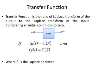


![Calculation of the Transfer Function
• Consider the following ODE where y(t) is input of the system and
x(t) is the output.
• or
A
d 2 x(t )
dy(t )
C
dt
dt 2
Ax' ' (t )
dx(t )
B
dt
Cy ' (t ) Bx' (t )
• Taking the Laplace transform on either sides
A[ s 2 X ( s ) sx( 0)
x' ( 0)]
C[ sY ( s )
y( 0)] B[ sX ( s )
x( 0)]
9](https://image.slidesharecdn.com/lecture-2transferfunction-140304142008-phpapp02/85/Lecture-2-transfer-function-9-320.jpg)
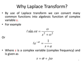
![Calculation of the Transfer Function
A[ s 2 X ( s ) sx( 0)
x' ( 0)]
C[ sY ( s )
y( 0)] B[ sX ( s )
x( 0)]
• Considering Initial conditions to zero in order to find the transfer
function of the system
As 2 X ( s )
CsY ( s ) BsX ( s )
• Rearranging the above equation
As 2 X ( s ) BsX ( s )
X ( s )[ As 2
X (s)
Y (s)
Bs ]
Cs
As 2
Bs
CsY ( s )
CsY ( s )
C
As B
10](https://image.slidesharecdn.com/lecture-2transferfunction-140304142008-phpapp02/85/Lecture-2-transfer-function-10-320.jpg)
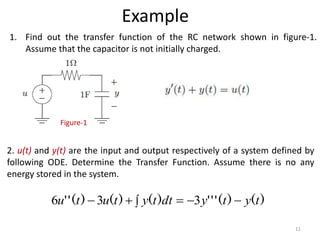
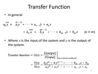
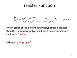
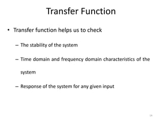

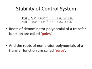

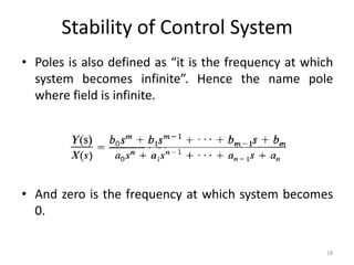


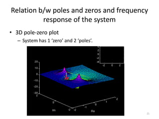
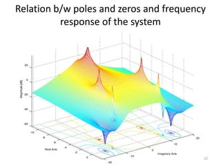
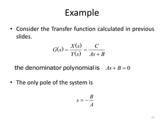
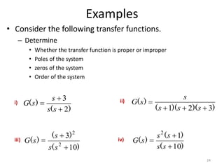
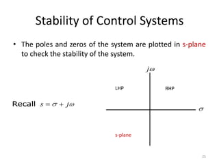

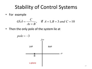
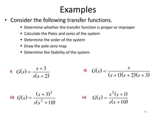


This document provides an overview of transfer functions and stability analysis of linear time-invariant (LTI) systems. It discusses how the Laplace transform can be used to represent signals as algebraic functions and calculate transfer functions as the ratio of the Laplace transforms of the output and input. Poles and zeros are introduced as important factors for stability. A system is stable if all its poles reside in the left half of the s-plane and unstable if any pole resides in the right half-plane. Examples are provided to demonstrate calculating transfer functions from differential equations and analyzing stability based on pole locations.


![Circuit Network Analysis - [Chapter5] Transfer function, frequency response, ...](https://cdn.slidesharecdn.com/ss_thumbnails/ch5-150613063859-lva1-app6891-thumbnail.jpg?width=640&height=640&fit=bounds)


