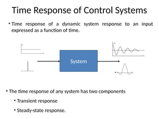
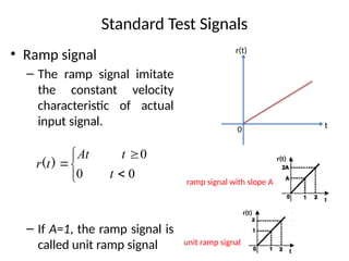
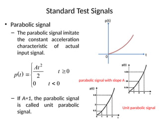
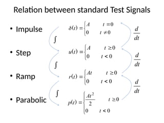
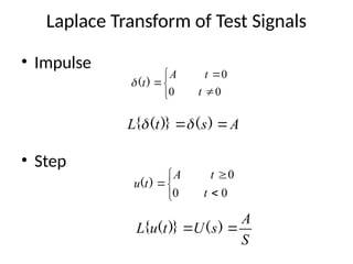
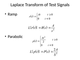
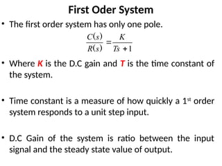
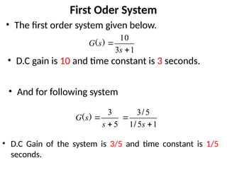
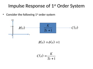
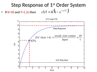
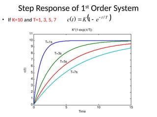
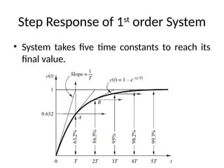
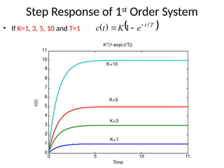
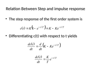
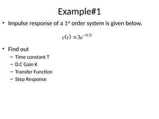
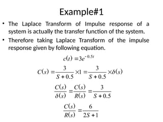
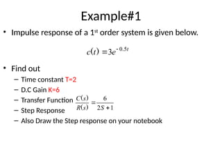
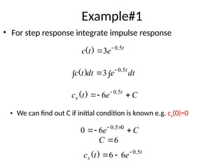
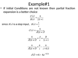
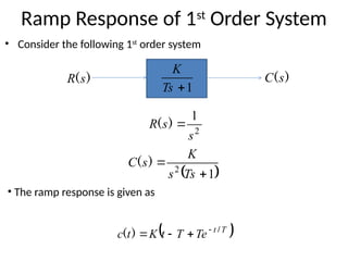
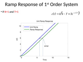
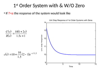
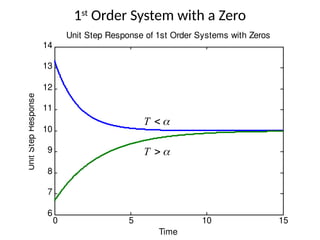
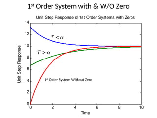
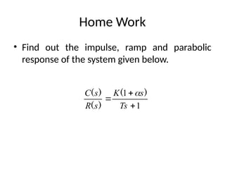
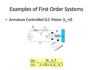
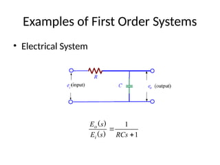
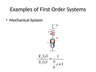
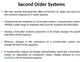
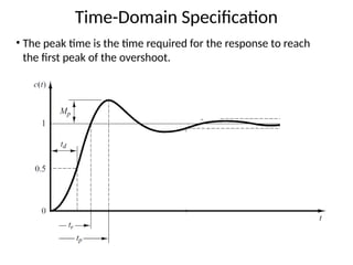
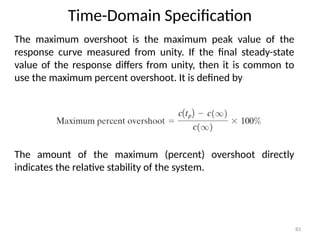
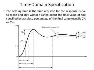
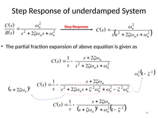
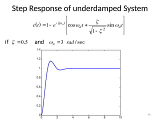
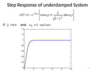
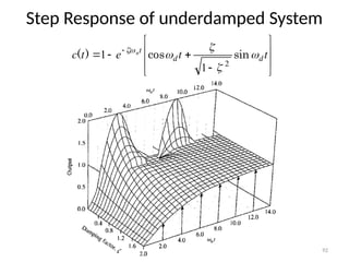
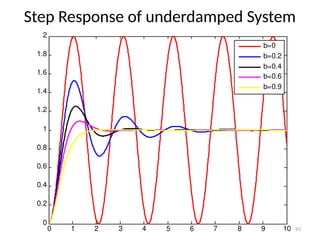
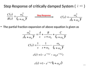
1
Dr. Imtiaz Hussain
Associate Professor
Mehran University of Engineering & Technology Jamshoro, Pakistan
email: imtiaz.hussain@faculty.muet.edu.pk
URL :http://imtiazhussainkalwar.weebly.com/
Lecture-5
Transient Response Analysis Of Control Systems
Note: I do not claim any originality in these lectures. The contents of this presentation are
mostly taken from the book of Ogatta, Norman Nise, Bishop and B C. Kuo and various other
internet sources.
Control Systems (CS)
6th
Semester 14ES (SEC-I)
Outline
• Introduction
• Standard Test Signals
• Transient Response of 1st
Order Systems
• Transient Response of 2nd
Order Systems
• S-Plane
• Transient Response Specifications of 2md order System
• Examples
Introduction
• In time-domain analysis the response of a dynamic system to an
input is expressed as a function of time.
• It is possible to compute the time response of a system if the
nature of input and the mathematical model of the system are
known.
• Usually, the input signals to control systems are not known fully
ahead of time.
• For example, in a radar tracking system, the position and the
speed of the target to be tracked may vary in a random fashion.
• It is therefore difficult to express the actual input signals
mathematically by simple equations.
Standard Test Signals
• The characteristics of actual input signals are a sudden
shock, a sudden change, a constant velocity, and constant
acceleration.
• The dynamic behavior of a system is therefore judged and
compared under application of standard test signals – an
impulse, a step, a constant velocity, and constant
acceleration.
• Another standard signal of great importance is a sinusoidal
signal.
Time Response of Control Systems
System
• The time response of any system has two components
• Transient response
• Steady-state response.
• Time response of a dynamic system response to an input
expressed as a function of time.
Time Response of Control Systems
• When the response of the system is changed form rest or
equilibrium it takes some time to settle down.
• Transient response is the response of a system from rest or
equilibrium to steady state.
0 2 4 6 8 10 12 14 16 18 20
0
1
2
3
4
5
6
x 10
-3
Step Response
Time (sec)
Amplitude
Response
Step Input
Transient Response
Steady
State
Response
• The response of the
system after the transient
response is called steady
state response.
Time Response of Control Systems
• Transient response depend upon the system poles only and not
on the type of input.
• It is therefore sufficient to analyze the transient response using a
step input.
• The steady-state response depends on system dynamics and the
input quantity.
• It is then examined using different test signals by final value
theorem.
Standard Test Signals
• Impulse signal
– The impulse signal imitate the
sudden shock characteristic of
actual input signal.
– If A=1, the impulse signal is
called unit impulse signal.
0 t
δ(t)
A






0
0
0
t
t
A
t)
(

Standard Test Signals
• Step signal
– The step signal imitate
the sudden change
characteristic of actual
input signal.
– If A=1, the step signal is
called unit step signal






0
0
0
t
t
A
t
u )
( 0 t
u(t)
A
Standard Test Signals
• Ramp signal
– The ramp signal imitate
the constant velocity
characteristic of actual
input signal.
– If A=1, the ramp signal is
called unit ramp signal






0
0
0
t
t
At
t
r )
(
0 t
r(t)
r(t)
unit ramp signal
r(t)
ramp signal with slope A
Standard Test Signals
• Parabolic signal
– The parabolic signal imitate
the constant acceleration
characteristic of actual
input signal.
– If A=1, the parabolic signal
is called unit parabolic
signal.








0
0
0
2
2
t
t
At
t
p )
(
0 t
p(t)
parabolic signal with slope A
p(t)
Unit parabolic signal
p(t)
Relation between standard Test Signals
• Impulse
• Step
• Ramp
• Parabolic






0
0
0
t
t
A
t)
(







0
0
0
t
t
A
t
u )
(






0
0
0
t
t
At
t
r )
(








0
0
0
2
2
t
t
At
t
p )
(


 dt
d
dt
d
dt
d
Laplace Transform of Test Signals
• Impulse
• Step






0
0
0
t
t
A
t)
(

A
s
t
L 
 )
(
)}
(
{ 







0
0
0
t
t
A
t
u )
(
S
A
s
U
t
u
L 
 )
(
)}
(
{
Laplace Transform of Test Signals
• Ramp
• Parabolic
2
s
A
s
R
t
r
L 
 )
(
)}
(
{
3
2
S
A
s
P
t
p
L 
 )
(
)}
(
{






0
0
0
t
t
At
t
r )
(








0
0
0
2
2
t
t
At
t
p )
(
First Oder System
• The first order system has only one pole.
• Where K is the D.C gain and T is the time constant of
the system.
• Time constant is a measure of how quickly a 1st
order
system responds to a unit step input.
• D.C Gain of the system is ratio between the input
signal and the steady state value of output.
1


Ts
K
s
R
s
C
)
(
)
(
First Oder System
• The first order system given below.
1
3
10


s
s
G )
(
5
3


s
s
G )
(
1
5
1
5
3


s
/
/
• D.C gain is 10 and time constant is 3 seconds.
• And for following system
• D.C Gain of the system is 3/5 and time constant is 1/5
seconds.
Impulse Response of 1st
Order System
• Consider the following 1st
order system
1

Ts
K
)
(s
C
)
(s
R
0
t
δ(t)
1
1

 )
(
)
( s
s
R 
1


Ts
K
s
C )
(
Impulse Response of 1st
Order System
• Re-arrange above equation as
1


Ts
K
s
C )
(
T
s
T
K
s
C
/
/
)
(
1


T
t
e
T
K
t
c /
)
( 

• In order represent the response of the system in time domain
we need to compute inverse Laplace transform of the above
equation.
at
Ce
a
s
C
L 









1
Impulse Response of 1st
Order System
T
t
e
T
K
t
c /
)
( 

• If K=3 and T=2s then
0 2 4 6 8 10
0
0.5
1
1.5
Time
c(t)
K/T*exp(-t/T)
Step Response of 1st
Order System
• Consider the following 1st
order system
1

Ts
K
)
(s
C
)
(s
R
s
s
U
s
R
1

 )
(
)
(
 
1


Ts
s
K
s
C )
(
1



Ts
KT
s
K
s
C )
(
• In order to find out the inverse Laplace of the above equation, we
need to break it into partial fraction expansion
Forced Response Natural Response
Step Response of 1st
Order System
• Taking Inverse Laplace of above equation









1
1
Ts
T
s
K
s
C )
(
 
T
t
e
t
u
K
t
c /
)
(
)
( 


• Where u(t)=1
 
T
t
e
K
t
c /
)
( 

 1
  K
e
K
t
c 632
0
1 1
.
)
( 

 
• When t=T
Step Response of 1st
Order System
• If K=10 and T=1.5s then  
T
t
e
K
t
c /
)
( 

 1
0 1 2 3 4 5 6 7 8 9 10
0
1
2
3
4
5
6
7
8
9
10
11
Time
c(t)
K*(1-exp(-t/T))
Unit Step Input
Step Response
1
10



Input
output
state
steady
K
Gain
C
D.
%
63
Step Response of 1st
Order System
• If K=10 and T=1, 3, 5, 7  
T
t
e
K
t
c /
)
( 

 1
0 5 10 15
0
1
2
3
4
5
6
7
8
9
10
11
Time
c(t)
K*(1-exp(-t/T))
T=3s
T=5s
T=7s
T=1s
Step Response of 1st
order System
• System takes five time constants to reach its
final value.
Step Response of 1st
Order System
• If K=1, 3, 5, 10 and T=1  
T
t
e
K
t
c /
)
( 

 1
0 5 10 15
0
1
2
3
4
5
6
7
8
9
10
11
Time
c(t)
K*(1-exp(-t/T))
K=1
K=3
K=5
K=10
Relation Between Step and impulse response
• The step response of the first order system is
• Differentiating c(t) with respect to t yields
  T
t
T
t
Ke
K
e
K
t
c /
/
)
( 




 1
 
T
t
Ke
K
dt
d
dt
t
dc /
)
( 


T
t
e
T
K
dt
t
dc /
)
( 

Example#1
• Impulse response of a 1st
order system is given below.
• Find out
– Time constant T
– D.C Gain K
– Transfer Function
– Step Response
t
e
t
c 5
0
3 .
)
( 

Example#1
• The Laplace Transform of Impulse response of a
system is actually the transfer function of the system.
• Therefore taking Laplace Transform of the impulse
response given by following equation.
t
e
t
c 5
0
3 .
)
( 

)
(
.
.
)
( s
S
S
s
C 






5
0
3
1
5
0
3
5
0
3
.
)
(
)
(
)
(
)
(



S
s
R
s
C
s
s
C

1
2
6


S
s
R
s
C
)
(
)
(
Example#1
• Impulse response of a 1st
order system is given below.
• Find out
– Time constant T=2
– D.C Gain K=6
– Transfer Function
– Step Response
– Also Draw the Step response on your notebook
t
e
t
c 5
0
3 .
)
( 

1
2
6


S
s
R
s
C
)
(
)
(
Example#1
• For step response integrate impulse response
t
e
t
c 5
0
3 .
)
( 

dt
e
dt
t
c t



 5
0
3 .
)
(
C
e
t
c t
s 

  5
0
6 .
)
(
• We can find out C if initial condition is known e.g. cs(0)=0
C
e 

 
 0
5
0
6
0 .
6

C
t
s e
t
c 5
0
6
6 .
)
( 


Example#1
• If initial Conditions are not known then partial fraction
expansion is a better choice
1
2
6


S
s
R
s
C
)
(
)
(
 
1
2
6


S
s
s
C )
(
  1
2
1
2
6



 s
B
s
A
S
s
s
s
R
s
R
1

)
(
,
)
( input
step
a
is
since
  5
0
6
6
1
2
6
.



 s
s
S
s
t
e
t
c 5
0
6
6 .
)
( 


Ramp Response of 1st
Order System
• Consider the following 1st
order system
1

Ts
K
)
(s
C
)
(s
R
2
1
s
s
R 
)
(
 
1
2


Ts
s
K
s
C )
(
• The ramp response is given as
 
T
t
Te
T
t
K
t
c /
)
( 



0 5 10 15
0
2
4
6
8
10
Time
c(t)
Unit Ramp Response
Unit Ramp
Ramp Response
Ramp Response of 1st
Order System
• If K=1 and T=1
 
T
t
Te
T
t
K
t
c /
)
( 



error
0 5 10 15
0
2
4
6
8
10
Time
c(t)
Unit Ramp Response
Unit Ramp
Ramp Response
Ramp Response of 1st
Order System
• If K=1 and T=3
 
T
t
Te
T
t
K
t
c /
)
( 



error
Parabolic Response of 1st
Order System
• Consider the following 1st
order system
1

Ts
K
)
(s
C
)
(s
R
3
1
s
s
R 
)
(
 
1
3


Ts
s
K
s
C )
(
• Do it yourself
Therefore,
Practical Determination of Transfer Function
of 1st
Order Systems
• Often it is not possible or practical to obtain a system's
transfer function analytically.
• Perhaps the system is closed, and the component parts are
not easily identifiable.
• The system's step response can lead to a representation even
though the inner construction is not known.
• With a step input, we can measure the time constant and the
steady-state value, from which the transfer function can be
calculated.
Practical Determination of Transfer
Function of 1st
Order Systems
• If we can identify T and K from laboratory testing we can
obtain the transfer function of the system.
1


Ts
K
s
R
s
C
)
(
)
(
Practical Determination of Transfer Function
of 1st
Order Systems
• For example, assume the unit
step response given in figure.
• From the response, we can
measure the time constant, that
is, the time for the amplitude to
reach 63% of its final value.
• Since the final value is about
0.72 the time constant is
evaluated where the curve
reaches 0.63 x 0.72 = 0.45, or
about 0.13 second.
T=0.13s
K=0.72
• K is simply steady state value.
• Thus transfer function is
obtained as:
7
7
5
5
1
13
0
72
0
.
.
.
.
)
(
)
(




s
s
s
R
s
C
1st
Order System with a Zero
• Zero of the system lie at -1/α and pole at -1/T.
1
1



Ts
s
K
s
R
s
C )
(
)
(
)
( 
 
1
1



Ts
s
s
K
s
C
)
(
)
(

• Step response of the system would be:
 
1




Ts
T
K
s
K
s
C
)
(
)
(

T
t
e
T
T
K
K
t
c /
)
(
)
( 


 
 
T
t
e
K
t
c /
)
( 

 1
1st
Order System with & W/O Zero
1
1



Ts
s
K
s
R
s
C )
(
)
(
)
( 
T
t
e
T
T
K
K
t
c /
)
(
)
( 


 
 
T
t
e
K
t
c /
)
( 

 1
1


Ts
K
s
R
s
C
)
(
)
(
• If T>α the response will be same
T
t
e
n
T
K
K
t
c /
)
(
)
( 










  T
t
e
T
Kn
K
t
c /
)
( 1
1st
Order System with & W/O Zero
• If T>α the response of the system would look like
0 5 10 15
6.5
7
7.5
8
8.5
9
9.5
10
Time
c(t)
Unit Step Response
1
3
2
1
10



s
s
s
R
s
C )
(
)
(
)
(
3
3
2
3
10
10 /
)
(
)
( t
e
t
c 



1st
Order System with & W/O Zero
• If T<α the response of the system would look like
1
5
1
2
1
10



s
s
s
R
s
C
.
)
(
)
(
)
(
5
1
1
2
5
1
10
10 .
/
)
(
.
)
( t
e
t
c 



0 5 10 15
9
10
11
12
13
14
Time
Unit
Step
Response
Unit Step Response of 1st Order Systems with Zeros
1st
Order System with a Zero
0 5 10 15
6
7
8
9
10
11
12
13
14
Time
Unit
Step
Response Unit Step Response of 1st Order Systems with Zeros


T


T
1st
Order System with & W/O Zero
0 2 4 6 8 10
0
2
4
6
8
10
12
14
Time
Unit
Step
Response Unit Step Response of 1st Order Systems with Zeros


T


T
1st
Order System Without Zero
Home Work
• Find out the impulse, ramp and parabolic
response of the system given below.
1
1



Ts
s
K
s
R
s
C )
(
)
(
)
( 
Example#2
• A thermometer requires 1 min to indicate 98% of the
response to a step input. Assuming the thermometer to
be a first-order system, find the time constant.
• If the thermometer is placed in a bath, the temperature
of which is changing linearly at a rate of 10°min, how
much error does the thermometer show?
PZ-map and Step Response
1


Ts
K
s
R
s
C
)
(
)
(
-1
-2
-3
δ
jω
1
10


s
s
R
s
C
)
(
)
(
s
T 1

PZ-map and Step Response
1


Ts
K
s
R
s
C
)
(
)
(
-1
-2
-3
δ
jω
2
10


s
s
R
s
C
)
(
)
( s
T 5
0.

1
5
0
5


s
s
R
s
C
.
)
(
)
(
PZ-map and Step Response
1


Ts
K
s
R
s
C
)
(
)
(
-1
-2
-3
δ
jω
3
10


s
s
R
s
C
)
(
)
( s
T 33
0.

1
33
0
3
3


s
s
R
s
C
.
.
)
(
)
(
Comparison
1
1


s
s
R
s
C
)
(
)
(
10
1


s
s
R
s
C
)
(
)
(
Step Response
Time (sec)
Amplitude
0 1 2 3 4 5 6
0
0.2
0.4
0.6
0.8
1
0 0.1 0.2 0.3 0.4 0.5 0.6
0
0.02
0.04
0.06
0.08
0.1
Step Response
Time (sec)
Amplitude
First Order System With Delays
• Following transfer function is the generic
representation of 1st
order system with time
lag.
• Where td is the delay time.
d
st
e
Ts
K
s
R
s
C 


1
)
(
)
(
First Order System With Delays
d
st
e
Ts
K
s
R
s
C 


1
)
(
)
(
1
Unit Step
Step Response
t
td
First Order System With Delays
s
e
s
s
R
s
C 2
1
3
10 


)
(
)
(
0 5 10 15
0
2
4
6
8
10
Step Response
Time (sec)
Amplitude
s
td 2

s
T 3

10

K
Examples of First Order Systems
• Armature Controlled D.C Motor (La=0)
 
 
a
b
t
a
t
R
K
K
B
Js
R
K
U(s)
Ω(s)



u
ia
T
Ra La
J

B
eb
Vf
=constant
Examples of First Order Systems
• Electrical System
1
1


RCs
s
E
s
E
i
o
)
(
)
(
Examples of First Order Systems
• Mechanical System
1
1


s
k
b
s
X
s
X
i
o
)
(
)
(
57
Second Order Systems
• We have already discussed the affect of location of poles and zeros on
the transient response of 1st
order systems.
• Compared to the simplicity of a first-order system, a second-order system
exhibits a wide range of responses that must be analyzed and described.
• Varying a first-order system's parameter (T, K) simply changes the speed
and offset of the response
• Whereas, changes in the parameters of a second-order system can
change the form of the response.
• A second-order system can display characteristics much like a first-order
system or, depending on component values, display damped or pure
oscillations for its transient response.
58
Second Order Systems
• A general second-order system is characterized by the
following transfer function.
2
2
2
2 n
n
n
s
s
s
R
s
C






)
(
)
(
un-damped natural frequency of the second order system, which is
the frequency of oscillation of the system without damping.
n

damping ratio of the second order system, which is a measure
of the degree of resistance to change in the system output.

59
Example#3
4
2
4
2



s
s
s
R
s
C
)
(
)
(
• Determine the un-damped natural frequency and damping ratio
of the following second order system.
4
2

n

2
2
2
2 n
n
n
s
s
s
R
s
C






)
(
)
(
• Compare the numerator and denominator of the given transfer
function with the general 2nd
order transfer function.
sec
/
rad
n 2

 
s
s
n 2
2 
 
4
2
2 2
2
2




 s
s
s
s n
n 

5
0.

 
1

 n

60
Second Order Systems
2
2
2
2 n
n
n
s
s
s
R
s
C






)
(
)
(
• Two poles of the system are
1
1
2
2














n
n
n
n
61
Second Order Systems
• According the value of , a second-order system can be set into one
of the four categories:
1
1
2
2














n
n
n
n

1. Overdamped - when the system has two real distinct poles ( >1).

-a
-b
-c
δ
jω
62
Second Order Systems
• According the value of , a second-order system can be set into one
of the four categories:
1
1
2
2














n
n
n
n

2. Underdamped - when the system has two complex conjugate poles (0 < <1)

-a
-b
-c
δ
jω
63
Second Order Systems
• According the value of , a second-order system can be set into one
of the four categories:
1
1
2
2














n
n
n
n

3. Undamped - when the system has two imaginary poles ( = 0).

-a
-b
-c
δ
jω
64
Second Order Systems
• According the value of , a second-order system can be set into one
of the four categories:
1
1
2
2














n
n
n
n

4. Critically damped - when the system has two real but equal poles ( = 1).

-a
-b
-c
δ
jω
65
S-Plane
δ
jω
• Natural Undamped Frequency.
n

• Distance from the origin of s-
plane to pole is natural
undamped frequency in
rad/sec.
66
S-Plane
δ
jω
• Let us draw a circle of radius 3 in s-plane.
3
-3
-3
3
• If a pole is located anywhere on the circumference of the circle the
natural undamped frequency would be 3 rad/sec.
67
S-Plane
δ
jω
• Therefore the s-plane is divided into Constant Natural
Undamped Frequency (ωn) Circles.
68
S-Plane
δ
jω
• Damping ratio.
• Cosine of the angle between
vector connecting origin and
pole and –ve real axis yields
damping ratio.


 cos

69
S-Plane
δ
jω
• For Underdamped system therefore,


90
0 
  1
0 
 
70
S-Plane
δ
jω
• For Undamped system therefore,

90

 0


71
S-Plane
δ
jω
• For overdamped and critically damped systems
therefore,

0


0


72
S-Plane
δ
jω
• Draw a vector connecting origin of s-plane and some point P.
P

45
707
0
45 .
cos 
 

73
S-Plane
δ
jω
• Therefore, s-plane is divided into sections of constant damping
ratio lines.
74
S-Plane
-4 -3.5 -3 -2.5 -2 -1.5 -1 -0.5 0
-1.5
-1
-0.5
0
0.5
1
1.5
0.22
0.42
0.6
0.74
0.84
0.91
0.96
0.99
0.22
0.42
0.6
0.74
0.84
0.91
0.96
0.99
0.5
1
1.5
2
2.5
3
3.5
4
Pole-Zero Map
-1
Imaginary
Axis
(seconds
-1
)
75
Example-4
• Determine the natural frequency
and damping ratio of the poles
from the given pz-map.
• Also determine the transfer
function of the system and state
whether system is
underdamped, overdamped,
undamped or critically damped.
-3 -2.5 -2 -1.5 -1 -0.5 0
-3
-2
-1
0
1
2
3
0.42
0.56
0.7
0.82
0.91
0.975
0.5
1
1.5
2
2.5
3
0.5
1
1.5
2
2.5
3
0.14
0.28
0.42
0.56
0.7
0.82
0.91
0.975
0.14
0.28
Pole-Zero Map
Imaginary
Axis
(seconds
-1
)
76
Example-5
• The natural frequency of closed
loop poles of 2nd
order system is 2
rad/sec and damping ratio is 0.5.
• Determine the location of closed
loop poles so that the damping
ratio remains same but the natural
undamped frequency is doubled.
4
2
4
2 2
2
2
2






s
s
s
s
s
R
s
C
n
n
n



)
(
)
(
-2 -1.5 -1 -0.5 0
-3
-2
-1
0
1
2
3
0.28
0.38
0.5
0.64
0.8
0.94
0.5
1
1.5
2
2.5
3
0.5
1
1.5
2
2.5
3
0.08
0.17
0.28
0.38
0.5
0.64
0.8
0.94
0.08
0.17
Pole-Zero Map
Real Axis
Imaginary
Axis
77
Example-5
Determine the location of closed loop poles so that the damping ratio remains same
but the natural undamped frequency is doubled.
-8 -6 -4 -2 0 2 4
-5
-4
-3
-2
-1
0
1
2
3
4
5
0.5
0.5
2
4
Pole-Zero Map
Imaginary
Axis
78
S-Plane

1
1
2
2














n
n
n
n
Time-Domain Specification
79
For 0< <1 and ωn > 0, the 2nd
order system’s response due to a
unit step input looks like

Time-Domain Specification
80
• The delay (td) time is the time required for the response to
reach half the final value the very first time.
Time-Domain Specification
• The rise time is the time required for the response to rise from 10%
to 90%, 5% to 95%, or 0% to 100% of its final value.
• For underdamped second order systems, the 0% to 100% rise time is
normally used. For overdamped systems, the 10% to 90% rise time is
commonly used.
Time-Domain Specification
82
• The peak time is the time required for the response to reach
the first peak of the overshoot.
82
82
Time-Domain Specification
83
The maximum overshoot is the maximum peak value of the
response curve measured from unity. If the final steady-state
value of the response differs from unity, then it is common to
use the maximum percent overshoot. It is defined by
The amount of the maximum (percent) overshoot directly
indicates the relative stability of the system.
Time-Domain Specification
84
• The settling time is the time required for the response curve
to reach and stay within a range about the final value of size
specified by absolute percentage of the final value (usually 2%
or 5%).
85
Step Response of underdamped System
2
2
2
2
2
2
2
2
1
n
n
n
n
n
s
s
s
s
s
C














)
(
• The partial fraction expansion of above equation is given as
2
2
2
2
1
n
n
n
s
s
s
s
s
C








)
(
 2
2 n
s 

 
2
2
1 
 
n
   
2
2
2
1
2
1










n
n
n
s
s
s
s
C )
(
2
2
2
2 n
n
n
s
s
s
R
s
C






)
(
)
(
 
2
2
2
2 n
n
n
s
s
s
s
C






)
(
Step Response
86
Step Response of underdamped System
• Above equation can be written as
   
2
2
2
1
2
1










n
n
n
s
s
s
s
C )
(
  2
2
2
1
d
n
n
s
s
s
s
C








)
(
2
1 

 
 n
d
• Where , is the frequency of transient oscillations
and is called damped frequency.
• The inverse Laplace transform of above equation can be obtained
easily if C(s) is written in the following form:
    2
2
2
2
1
d
n
n
d
n
n
s
s
s
s
s
C














)
(
87
Step Response of underdamped System
    2
2
2
2
1
d
n
n
d
n
n
s
s
s
s
s
C














)
(
    2
2
2
2
2
2
1
1
1
d
n
n
d
n
n
s
s
s
s
s
C



















)
(
    2
2
2
2
2
1
1
d
n
d
d
n
n
s
s
s
s
s
C

















)
(
t
e
t
e
t
c d
t
d
t n
n



 

sin
cos
)
( 





2
1
1
88
Step Response of underdamped System
t
e
t
e
t
c d
t
d
t n
n



 

sin
cos
)
( 





2
1
1











 
t
t
e
t
c d
d
t
n





sin
cos
)
(
2
1
1
n
n
d






 2
1
• When 0


t
t
c n

cos
)
( 
1
89
Step Response of underdamped System











 
t
t
e
t
c d
d
t
n





sin
cos
)
(
2
1
1
sec
/
. rad
n
and
if 3
1
0 
 

0 2 4 6 8 10
0
0.2
0.4
0.6
0.8
1
1.2
1.4
1.6
1.8
90
Step Response of underdamped System











 
t
t
e
t
c d
d
t
n





sin
cos
)
(
2
1
1
sec
/
. rad
n
and
if 3
5
0 
 

0 2 4 6 8 10
0
0.2
0.4
0.6
0.8
1
1.2
1.4
91
Step Response of underdamped System











 
t
t
e
t
c d
d
t
n





sin
cos
)
(
2
1
1
sec
/
. rad
n
and
if 3
9
0 
 

0 2 4 6 8 10
0
0.2
0.4
0.6
0.8
1
1.2
1.4
92
Step Response of underdamped System











 
t
t
e
t
c d
d
t
n





sin
cos
)
(
2
1
1
93
Step Response of underdamped System
0 1 2 3 4 5 6 7 8 9 10
0
0.2
0.4
0.6
0.8
1
1.2
1.4
1.6
1.8
2
b=0
b=0.2
b=0.4
b=0.6
b=0.9
94
Step Response of underdamped System
0 1 2 3 4 5 6 7 8 9 10
0
0.2
0.4
0.6
0.8
1
1.2
1.4
wn=0.5
wn=1
wn=1.5
wn=2
wn=2.5
95
Time Domain Specifications
n
s T
t

4
4 

n
s T
t

3
3 
 100
2
1






e
M p
2
1 







n
d
p
t
2
1 











n
d
r
t
Rise Time Peak Time
Settling Time (2%)
Settling Time (5%)
Maximum Overshoot
96
Example#6
• Consider the system shown in following figure, where
damping ratio is 0.6 and natural undamped frequency is 5
rad/sec. Obtain the rise time tr, peak time tp, maximum
overshoot Mp, and settling time 2% and 5% criterion ts when
the system is subjected to a unit-step input.
97
Example#6
n
s T
t

4
4 

100
2
1






e
M p
d
p
t



d
r
t


 

Rise Time Peak Time
Settling Time (2%) Maximum Overshoot
n
s T
t

3
3 

Settling Time (5%)
98
Example#6
d
r
t


 

Rise Time

2
1
141
3






n
r
t
.
rad
93
0
1 2
1
.
)
(
tan 

 
n
n




s
tr 55
0
6
0
1
5
93
0
141
3
2
.
.
.
.




99
Example#6
n
s
t

4

d
p
t



Peak Time
Settling Time (2%)
n
s
t

3

Settling Time (5%)
s
tp 785
0
4
141
3
.
.


s
ts 33
1
5
6
0
4
.
.



s
ts 1
5
6
0
3



.
100
Example#6
100
2
1






e
M p
Maximum Overshoot
100
2
6
0
1
6
0
141
3

 


.
.
.
e
M p
100
095
0 
 .
p
M
%
.5
9

p
M
101
Example#6
Step Response
Time (sec)
Amplitude
0 0.2 0.4 0.6 0.8 1 1.2 1.4 1.6
0
0.2
0.4
0.6
0.8
1
1.2
1.4
Mp
Rise Time
102
Example#7
• For the system shown in Figure-(a), determine the values of gain K
and velocity-feedback constant Kh so that the maximum overshoot
in the unit-step response is 0.2 and the peak time is 1 sec. With
these values of K and Kh, obtain the rise time and settling time.
Assume that J=1 kg-m2
and B=1 N-m/rad/sec.
103
Example#7
104
Example#7
Nm/rad/sec
and
Since 1
1 2

 B
kgm
J
K
s
KK
s
K
s
R
s
C
h 



)
(
)
(
)
(
1
2
2
2
2
2 n
n
n
s
s
s
R
s
C






)
(
)
(
• Comparing above T.F with general 2nd
order T.F
K
n 

K
KKh
2
1 )
( 


105
Example#7
• Maximum overshoot is 0.2.
K
n 

K
KKh
2
1 )
( 


 
2
0
2
1
.
ln
)
ln( 




e
• The peak time is 1 sec
d
p
t



2
456
0
1
141
3
.
.


n

2
1
141
3
1

 

n
.
rad/sec
53
.
3

n

106
Example#7
K
n 

K
KKh
2
1 )
( 


rad/sec
96
.
3

n

K

53
3.
5
12
53
3 2
.
.


K
K
)
.
(
.
. h
K
5
12
1
5
12
2
456
0 


178
0.

h
K
107
Example#7
96
3.

n

n
s
t

4

n
s
t

3

2
1 






n
r
t
s
tr 65
0.
 s
ts 48
2.

s
ts 86
1.

108
Example#8
When the system shown in Figure(a) is subjected to a unit-step input,
the system output responds as shown in Figure(b). Determine the
values of a and c from the response curve.
)
( 1

cs
s
a
109
Example#9
Figure (a) shows a mechanical vibratory system. When 2 lb of force
(step input) is applied to the system, the mass oscillates, as shown in
Figure (b). Determine m, b, and k of the system from this response
curve.
110
Example#10
Given the system shown in following figure, find J and D to yield 20%
overshoot and a settling time of 2 seconds for a step input of torque
T(t).
111
Example#10
112
Example#10
113
Example # 11
• Ships at sea undergo
motion about their roll axis,
as shown in Figure. Fins
called stabilizers are used to
reduce this rolling motion.
The stabilizers can be
positioned by a closed-loop
roll control system that
consists of components,
such as fin actuators and
sensors, as well as the ship’s
roll dynamics.
114
Example # 11
• Assume the roll dynamics, which relates the roll-angle output, , to a
disturbance-torque input, TD(s), is
• Do the following:
a) Find the natural frequency, damping ratio, peak time, settling
time, rise time, and percent overshoot.
b) Find the analytical expression for the output response to a unit
step input.
115
Step Response of critically damped System ( )
• The partial fraction expansion of above equation is given as
 2
2
n
n
s
s
R
s
C




)
(
)
(
 2
2
n
n
s
s
s
C




)
(
Step Response
   2
2
2
n
n
n
n
s
C
s
B
s
A
s
s 









 2
1
1
n
n
n s
s
s
s
C


 




)
(
t
e
e
t
c t
n
t n
n 

 



1
)
(
 
t
e
t
c n
t
n




 
1
1
)
(
1


116
117
Example 12: Describe the nature of the second-order system
response via the value of the damping ratio for the systems with
transfer function
Second – Order System
12
8
12
)
(
.
1 2



s
s
s
G
16
8
16
)
(
.
2 2



s
s
s
G
20
8
20
)
(
.
3 2



s
s
s
G
Do them as your own
revision
118
Example-13
• For each of the transfer
functions find the locations of
the poles and zeros, plot them
on the s-plane, and then write
an expression for the general
form of the step response
without solving for the inverse
Laplace transform. State the
nature of each response
(overdamped, underdamped,
and so on).
119
Example-14
• Solve for x(t) in the system shown in Figure if f(t) is a unit step.
END OF LECTURE-5
To download this lecture visit
http://imtiazhussainkalwar.weebly.com/

lecture-5_transient_response_analysis_of_control_systems.pptx

  • 1.
    1 Dr. Imtiaz Hussain AssociateProfessor Mehran University of Engineering & Technology Jamshoro, Pakistan email: imtiaz.hussain@faculty.muet.edu.pk URL :http://imtiazhussainkalwar.weebly.com/ Lecture-5 Transient Response Analysis Of Control Systems Note: I do not claim any originality in these lectures. The contents of this presentation are mostly taken from the book of Ogatta, Norman Nise, Bishop and B C. Kuo and various other internet sources. Control Systems (CS) 6th Semester 14ES (SEC-I)
  • 2.
    Outline • Introduction • StandardTest Signals • Transient Response of 1st Order Systems • Transient Response of 2nd Order Systems • S-Plane • Transient Response Specifications of 2md order System • Examples
  • 3.
    Introduction • In time-domainanalysis the response of a dynamic system to an input is expressed as a function of time. • It is possible to compute the time response of a system if the nature of input and the mathematical model of the system are known. • Usually, the input signals to control systems are not known fully ahead of time. • For example, in a radar tracking system, the position and the speed of the target to be tracked may vary in a random fashion. • It is therefore difficult to express the actual input signals mathematically by simple equations.
  • 4.
    Standard Test Signals •The characteristics of actual input signals are a sudden shock, a sudden change, a constant velocity, and constant acceleration. • The dynamic behavior of a system is therefore judged and compared under application of standard test signals – an impulse, a step, a constant velocity, and constant acceleration. • Another standard signal of great importance is a sinusoidal signal.
  • 5.
    Time Response ofControl Systems System • The time response of any system has two components • Transient response • Steady-state response. • Time response of a dynamic system response to an input expressed as a function of time.
  • 6.
    Time Response ofControl Systems • When the response of the system is changed form rest or equilibrium it takes some time to settle down. • Transient response is the response of a system from rest or equilibrium to steady state. 0 2 4 6 8 10 12 14 16 18 20 0 1 2 3 4 5 6 x 10 -3 Step Response Time (sec) Amplitude Response Step Input Transient Response Steady State Response • The response of the system after the transient response is called steady state response.
  • 7.
    Time Response ofControl Systems • Transient response depend upon the system poles only and not on the type of input. • It is therefore sufficient to analyze the transient response using a step input. • The steady-state response depends on system dynamics and the input quantity. • It is then examined using different test signals by final value theorem.
  • 8.
    Standard Test Signals •Impulse signal – The impulse signal imitate the sudden shock characteristic of actual input signal. – If A=1, the impulse signal is called unit impulse signal. 0 t δ(t) A       0 0 0 t t A t) ( 
  • 9.
    Standard Test Signals •Step signal – The step signal imitate the sudden change characteristic of actual input signal. – If A=1, the step signal is called unit step signal       0 0 0 t t A t u ) ( 0 t u(t) A
  • 10.
    Standard Test Signals •Ramp signal – The ramp signal imitate the constant velocity characteristic of actual input signal. – If A=1, the ramp signal is called unit ramp signal       0 0 0 t t At t r ) ( 0 t r(t) r(t) unit ramp signal r(t) ramp signal with slope A
  • 11.
    Standard Test Signals •Parabolic signal – The parabolic signal imitate the constant acceleration characteristic of actual input signal. – If A=1, the parabolic signal is called unit parabolic signal.         0 0 0 2 2 t t At t p ) ( 0 t p(t) parabolic signal with slope A p(t) Unit parabolic signal p(t)
  • 12.
    Relation between standardTest Signals • Impulse • Step • Ramp • Parabolic       0 0 0 t t A t) (        0 0 0 t t A t u ) (       0 0 0 t t At t r ) (         0 0 0 2 2 t t At t p ) (    dt d dt d dt d
  • 13.
    Laplace Transform ofTest Signals • Impulse • Step       0 0 0 t t A t) (  A s t L   ) ( )} ( {         0 0 0 t t A t u ) ( S A s U t u L   ) ( )} ( {
  • 14.
    Laplace Transform ofTest Signals • Ramp • Parabolic 2 s A s R t r L   ) ( )} ( { 3 2 S A s P t p L   ) ( )} ( {       0 0 0 t t At t r ) (         0 0 0 2 2 t t At t p ) (
  • 15.
    First Oder System •The first order system has only one pole. • Where K is the D.C gain and T is the time constant of the system. • Time constant is a measure of how quickly a 1st order system responds to a unit step input. • D.C Gain of the system is ratio between the input signal and the steady state value of output. 1   Ts K s R s C ) ( ) (
  • 16.
    First Oder System •The first order system given below. 1 3 10   s s G ) ( 5 3   s s G ) ( 1 5 1 5 3   s / / • D.C gain is 10 and time constant is 3 seconds. • And for following system • D.C Gain of the system is 3/5 and time constant is 1/5 seconds.
  • 17.
    Impulse Response of1st Order System • Consider the following 1st order system 1  Ts K ) (s C ) (s R 0 t δ(t) 1 1   ) ( ) ( s s R  1   Ts K s C ) (
  • 18.
    Impulse Response of1st Order System • Re-arrange above equation as 1   Ts K s C ) ( T s T K s C / / ) ( 1   T t e T K t c / ) (   • In order represent the response of the system in time domain we need to compute inverse Laplace transform of the above equation. at Ce a s C L           1
  • 19.
    Impulse Response of1st Order System T t e T K t c / ) (   • If K=3 and T=2s then 0 2 4 6 8 10 0 0.5 1 1.5 Time c(t) K/T*exp(-t/T)
  • 20.
    Step Response of1st Order System • Consider the following 1st order system 1  Ts K ) (s C ) (s R s s U s R 1   ) ( ) (   1   Ts s K s C ) ( 1    Ts KT s K s C ) ( • In order to find out the inverse Laplace of the above equation, we need to break it into partial fraction expansion Forced Response Natural Response
  • 21.
    Step Response of1st Order System • Taking Inverse Laplace of above equation          1 1 Ts T s K s C ) (   T t e t u K t c / ) ( ) (    • Where u(t)=1   T t e K t c / ) (    1   K e K t c 632 0 1 1 . ) (     • When t=T
  • 22.
    Step Response of1st Order System • If K=10 and T=1.5s then   T t e K t c / ) (    1 0 1 2 3 4 5 6 7 8 9 10 0 1 2 3 4 5 6 7 8 9 10 11 Time c(t) K*(1-exp(-t/T)) Unit Step Input Step Response 1 10    Input output state steady K Gain C D. % 63
  • 23.
    Step Response of1st Order System • If K=10 and T=1, 3, 5, 7   T t e K t c / ) (    1 0 5 10 15 0 1 2 3 4 5 6 7 8 9 10 11 Time c(t) K*(1-exp(-t/T)) T=3s T=5s T=7s T=1s
  • 24.
    Step Response of1st order System • System takes five time constants to reach its final value.
  • 25.
    Step Response of1st Order System • If K=1, 3, 5, 10 and T=1   T t e K t c / ) (    1 0 5 10 15 0 1 2 3 4 5 6 7 8 9 10 11 Time c(t) K*(1-exp(-t/T)) K=1 K=3 K=5 K=10
  • 26.
    Relation Between Stepand impulse response • The step response of the first order system is • Differentiating c(t) with respect to t yields   T t T t Ke K e K t c / / ) (       1   T t Ke K dt d dt t dc / ) (    T t e T K dt t dc / ) (  
  • 27.
    Example#1 • Impulse responseof a 1st order system is given below. • Find out – Time constant T – D.C Gain K – Transfer Function – Step Response t e t c 5 0 3 . ) (  
  • 28.
    Example#1 • The LaplaceTransform of Impulse response of a system is actually the transfer function of the system. • Therefore taking Laplace Transform of the impulse response given by following equation. t e t c 5 0 3 . ) (   ) ( . . ) ( s S S s C        5 0 3 1 5 0 3 5 0 3 . ) ( ) ( ) ( ) (    S s R s C s s C  1 2 6   S s R s C ) ( ) (
  • 29.
    Example#1 • Impulse responseof a 1st order system is given below. • Find out – Time constant T=2 – D.C Gain K=6 – Transfer Function – Step Response – Also Draw the Step response on your notebook t e t c 5 0 3 . ) (   1 2 6   S s R s C ) ( ) (
  • 30.
    Example#1 • For stepresponse integrate impulse response t e t c 5 0 3 . ) (   dt e dt t c t     5 0 3 . ) ( C e t c t s     5 0 6 . ) ( • We can find out C if initial condition is known e.g. cs(0)=0 C e      0 5 0 6 0 . 6  C t s e t c 5 0 6 6 . ) (   
  • 31.
    Example#1 • If initialConditions are not known then partial fraction expansion is a better choice 1 2 6   S s R s C ) ( ) (   1 2 6   S s s C ) (   1 2 1 2 6     s B s A S s s s R s R 1  ) ( , ) ( input step a is since   5 0 6 6 1 2 6 .     s s S s t e t c 5 0 6 6 . ) (   
  • 32.
    Ramp Response of1st Order System • Consider the following 1st order system 1  Ts K ) (s C ) (s R 2 1 s s R  ) (   1 2   Ts s K s C ) ( • The ramp response is given as   T t Te T t K t c / ) (    
  • 33.
    0 5 1015 0 2 4 6 8 10 Time c(t) Unit Ramp Response Unit Ramp Ramp Response Ramp Response of 1st Order System • If K=1 and T=1   T t Te T t K t c / ) (     error
  • 34.
    0 5 1015 0 2 4 6 8 10 Time c(t) Unit Ramp Response Unit Ramp Ramp Response Ramp Response of 1st Order System • If K=1 and T=3   T t Te T t K t c / ) (     error
  • 35.
    Parabolic Response of1st Order System • Consider the following 1st order system 1  Ts K ) (s C ) (s R 3 1 s s R  ) (   1 3   Ts s K s C ) ( • Do it yourself Therefore,
  • 36.
    Practical Determination ofTransfer Function of 1st Order Systems • Often it is not possible or practical to obtain a system's transfer function analytically. • Perhaps the system is closed, and the component parts are not easily identifiable. • The system's step response can lead to a representation even though the inner construction is not known. • With a step input, we can measure the time constant and the steady-state value, from which the transfer function can be calculated.
  • 37.
    Practical Determination ofTransfer Function of 1st Order Systems • If we can identify T and K from laboratory testing we can obtain the transfer function of the system. 1   Ts K s R s C ) ( ) (
  • 38.
    Practical Determination ofTransfer Function of 1st Order Systems • For example, assume the unit step response given in figure. • From the response, we can measure the time constant, that is, the time for the amplitude to reach 63% of its final value. • Since the final value is about 0.72 the time constant is evaluated where the curve reaches 0.63 x 0.72 = 0.45, or about 0.13 second. T=0.13s K=0.72 • K is simply steady state value. • Thus transfer function is obtained as: 7 7 5 5 1 13 0 72 0 . . . . ) ( ) (     s s s R s C
  • 39.
    1st Order System witha Zero • Zero of the system lie at -1/α and pole at -1/T. 1 1    Ts s K s R s C ) ( ) ( ) (    1 1    Ts s s K s C ) ( ) (  • Step response of the system would be:   1     Ts T K s K s C ) ( ) (  T t e T T K K t c / ) ( ) (        T t e K t c / ) (    1
  • 40.
    1st Order System with& W/O Zero 1 1    Ts s K s R s C ) ( ) ( ) (  T t e T T K K t c / ) ( ) (        T t e K t c / ) (    1 1   Ts K s R s C ) ( ) ( • If T>α the response will be same T t e n T K K t c / ) ( ) (              T t e T Kn K t c / ) ( 1
  • 41.
    1st Order System with& W/O Zero • If T>α the response of the system would look like 0 5 10 15 6.5 7 7.5 8 8.5 9 9.5 10 Time c(t) Unit Step Response 1 3 2 1 10    s s s R s C ) ( ) ( ) ( 3 3 2 3 10 10 / ) ( ) ( t e t c    
  • 42.
    1st Order System with& W/O Zero • If T<α the response of the system would look like 1 5 1 2 1 10    s s s R s C . ) ( ) ( ) ( 5 1 1 2 5 1 10 10 . / ) ( . ) ( t e t c     0 5 10 15 9 10 11 12 13 14 Time Unit Step Response Unit Step Response of 1st Order Systems with Zeros
  • 43.
    1st Order System witha Zero 0 5 10 15 6 7 8 9 10 11 12 13 14 Time Unit Step Response Unit Step Response of 1st Order Systems with Zeros   T   T
  • 44.
    1st Order System with& W/O Zero 0 2 4 6 8 10 0 2 4 6 8 10 12 14 Time Unit Step Response Unit Step Response of 1st Order Systems with Zeros   T   T 1st Order System Without Zero
  • 45.
    Home Work • Findout the impulse, ramp and parabolic response of the system given below. 1 1    Ts s K s R s C ) ( ) ( ) ( 
  • 46.
    Example#2 • A thermometerrequires 1 min to indicate 98% of the response to a step input. Assuming the thermometer to be a first-order system, find the time constant. • If the thermometer is placed in a bath, the temperature of which is changing linearly at a rate of 10°min, how much error does the thermometer show?
  • 47.
    PZ-map and StepResponse 1   Ts K s R s C ) ( ) ( -1 -2 -3 δ jω 1 10   s s R s C ) ( ) ( s T 1 
  • 48.
    PZ-map and StepResponse 1   Ts K s R s C ) ( ) ( -1 -2 -3 δ jω 2 10   s s R s C ) ( ) ( s T 5 0.  1 5 0 5   s s R s C . ) ( ) (
  • 49.
    PZ-map and StepResponse 1   Ts K s R s C ) ( ) ( -1 -2 -3 δ jω 3 10   s s R s C ) ( ) ( s T 33 0.  1 33 0 3 3   s s R s C . . ) ( ) (
  • 50.
    Comparison 1 1   s s R s C ) ( ) ( 10 1   s s R s C ) ( ) ( Step Response Time (sec) Amplitude 01 2 3 4 5 6 0 0.2 0.4 0.6 0.8 1 0 0.1 0.2 0.3 0.4 0.5 0.6 0 0.02 0.04 0.06 0.08 0.1 Step Response Time (sec) Amplitude
  • 51.
    First Order SystemWith Delays • Following transfer function is the generic representation of 1st order system with time lag. • Where td is the delay time. d st e Ts K s R s C    1 ) ( ) (
  • 52.
    First Order SystemWith Delays d st e Ts K s R s C    1 ) ( ) ( 1 Unit Step Step Response t td
  • 53.
    First Order SystemWith Delays s e s s R s C 2 1 3 10    ) ( ) ( 0 5 10 15 0 2 4 6 8 10 Step Response Time (sec) Amplitude s td 2  s T 3  10  K
  • 54.
    Examples of FirstOrder Systems • Armature Controlled D.C Motor (La=0)     a b t a t R K K B Js R K U(s) Ω(s)    u ia T Ra La J  B eb Vf =constant
  • 55.
    Examples of FirstOrder Systems • Electrical System 1 1   RCs s E s E i o ) ( ) (
  • 56.
    Examples of FirstOrder Systems • Mechanical System 1 1   s k b s X s X i o ) ( ) (
  • 57.
    57 Second Order Systems •We have already discussed the affect of location of poles and zeros on the transient response of 1st order systems. • Compared to the simplicity of a first-order system, a second-order system exhibits a wide range of responses that must be analyzed and described. • Varying a first-order system's parameter (T, K) simply changes the speed and offset of the response • Whereas, changes in the parameters of a second-order system can change the form of the response. • A second-order system can display characteristics much like a first-order system or, depending on component values, display damped or pure oscillations for its transient response.
  • 58.
    58 Second Order Systems •A general second-order system is characterized by the following transfer function. 2 2 2 2 n n n s s s R s C       ) ( ) ( un-damped natural frequency of the second order system, which is the frequency of oscillation of the system without damping. n  damping ratio of the second order system, which is a measure of the degree of resistance to change in the system output. 
  • 59.
    59 Example#3 4 2 4 2    s s s R s C ) ( ) ( • Determine theun-damped natural frequency and damping ratio of the following second order system. 4 2  n  2 2 2 2 n n n s s s R s C       ) ( ) ( • Compare the numerator and denominator of the given transfer function with the general 2nd order transfer function. sec / rad n 2    s s n 2 2    4 2 2 2 2 2      s s s s n n   5 0.    1   n 
  • 60.
    60 Second Order Systems 2 2 2 2n n n s s s R s C       ) ( ) ( • Two poles of the system are 1 1 2 2               n n n n
  • 61.
    61 Second Order Systems •According the value of , a second-order system can be set into one of the four categories: 1 1 2 2               n n n n  1. Overdamped - when the system has two real distinct poles ( >1).  -a -b -c δ jω
  • 62.
    62 Second Order Systems •According the value of , a second-order system can be set into one of the four categories: 1 1 2 2               n n n n  2. Underdamped - when the system has two complex conjugate poles (0 < <1)  -a -b -c δ jω
  • 63.
    63 Second Order Systems •According the value of , a second-order system can be set into one of the four categories: 1 1 2 2               n n n n  3. Undamped - when the system has two imaginary poles ( = 0).  -a -b -c δ jω
  • 64.
    64 Second Order Systems •According the value of , a second-order system can be set into one of the four categories: 1 1 2 2               n n n n  4. Critically damped - when the system has two real but equal poles ( = 1).  -a -b -c δ jω
  • 65.
    65 S-Plane δ jω • Natural UndampedFrequency. n  • Distance from the origin of s- plane to pole is natural undamped frequency in rad/sec.
  • 66.
    66 S-Plane δ jω • Let usdraw a circle of radius 3 in s-plane. 3 -3 -3 3 • If a pole is located anywhere on the circumference of the circle the natural undamped frequency would be 3 rad/sec.
  • 67.
    67 S-Plane δ jω • Therefore thes-plane is divided into Constant Natural Undamped Frequency (ωn) Circles.
  • 68.
    68 S-Plane δ jω • Damping ratio. •Cosine of the angle between vector connecting origin and pole and –ve real axis yields damping ratio.    cos 
  • 69.
    69 S-Plane δ jω • For Underdampedsystem therefore,   90 0    1 0   
  • 70.
    70 S-Plane δ jω • For Undampedsystem therefore,  90   0  
  • 71.
    71 S-Plane δ jω • For overdampedand critically damped systems therefore,  0   0  
  • 72.
    72 S-Plane δ jω • Draw avector connecting origin of s-plane and some point P. P  45 707 0 45 . cos    
  • 73.
    73 S-Plane δ jω • Therefore, s-planeis divided into sections of constant damping ratio lines.
  • 74.
    74 S-Plane -4 -3.5 -3-2.5 -2 -1.5 -1 -0.5 0 -1.5 -1 -0.5 0 0.5 1 1.5 0.22 0.42 0.6 0.74 0.84 0.91 0.96 0.99 0.22 0.42 0.6 0.74 0.84 0.91 0.96 0.99 0.5 1 1.5 2 2.5 3 3.5 4 Pole-Zero Map -1 Imaginary Axis (seconds -1 )
  • 75.
    75 Example-4 • Determine thenatural frequency and damping ratio of the poles from the given pz-map. • Also determine the transfer function of the system and state whether system is underdamped, overdamped, undamped or critically damped. -3 -2.5 -2 -1.5 -1 -0.5 0 -3 -2 -1 0 1 2 3 0.42 0.56 0.7 0.82 0.91 0.975 0.5 1 1.5 2 2.5 3 0.5 1 1.5 2 2.5 3 0.14 0.28 0.42 0.56 0.7 0.82 0.91 0.975 0.14 0.28 Pole-Zero Map Imaginary Axis (seconds -1 )
  • 76.
    76 Example-5 • The naturalfrequency of closed loop poles of 2nd order system is 2 rad/sec and damping ratio is 0.5. • Determine the location of closed loop poles so that the damping ratio remains same but the natural undamped frequency is doubled. 4 2 4 2 2 2 2 2       s s s s s R s C n n n    ) ( ) ( -2 -1.5 -1 -0.5 0 -3 -2 -1 0 1 2 3 0.28 0.38 0.5 0.64 0.8 0.94 0.5 1 1.5 2 2.5 3 0.5 1 1.5 2 2.5 3 0.08 0.17 0.28 0.38 0.5 0.64 0.8 0.94 0.08 0.17 Pole-Zero Map Real Axis Imaginary Axis
  • 77.
    77 Example-5 Determine the locationof closed loop poles so that the damping ratio remains same but the natural undamped frequency is doubled. -8 -6 -4 -2 0 2 4 -5 -4 -3 -2 -1 0 1 2 3 4 5 0.5 0.5 2 4 Pole-Zero Map Imaginary Axis
  • 78.
  • 79.
    Time-Domain Specification 79 For 0<<1 and ωn > 0, the 2nd order system’s response due to a unit step input looks like 
  • 80.
    Time-Domain Specification 80 • Thedelay (td) time is the time required for the response to reach half the final value the very first time.
  • 81.
    Time-Domain Specification • Therise time is the time required for the response to rise from 10% to 90%, 5% to 95%, or 0% to 100% of its final value. • For underdamped second order systems, the 0% to 100% rise time is normally used. For overdamped systems, the 10% to 90% rise time is commonly used.
  • 82.
    Time-Domain Specification 82 • Thepeak time is the time required for the response to reach the first peak of the overshoot. 82 82
  • 83.
    Time-Domain Specification 83 The maximumovershoot is the maximum peak value of the response curve measured from unity. If the final steady-state value of the response differs from unity, then it is common to use the maximum percent overshoot. It is defined by The amount of the maximum (percent) overshoot directly indicates the relative stability of the system.
  • 84.
    Time-Domain Specification 84 • Thesettling time is the time required for the response curve to reach and stay within a range about the final value of size specified by absolute percentage of the final value (usually 2% or 5%).
  • 85.
    85 Step Response ofunderdamped System 2 2 2 2 2 2 2 2 1 n n n n n s s s s s C               ) ( • The partial fraction expansion of above equation is given as 2 2 2 2 1 n n n s s s s s C         ) (  2 2 n s     2 2 1    n     2 2 2 1 2 1           n n n s s s s C ) ( 2 2 2 2 n n n s s s R s C       ) ( ) (   2 2 2 2 n n n s s s s C       ) ( Step Response
  • 86.
    86 Step Response ofunderdamped System • Above equation can be written as     2 2 2 1 2 1           n n n s s s s C ) (   2 2 2 1 d n n s s s s C         ) ( 2 1      n d • Where , is the frequency of transient oscillations and is called damped frequency. • The inverse Laplace transform of above equation can be obtained easily if C(s) is written in the following form:     2 2 2 2 1 d n n d n n s s s s s C               ) (
  • 87.
    87 Step Response ofunderdamped System     2 2 2 2 1 d n n d n n s s s s s C               ) (     2 2 2 2 2 2 1 1 1 d n n d n n s s s s s C                    ) (     2 2 2 2 2 1 1 d n d d n n s s s s s C                  ) ( t e t e t c d t d t n n       sin cos ) (       2 1 1
  • 88.
    88 Step Response ofunderdamped System t e t e t c d t d t n n       sin cos ) (       2 1 1              t t e t c d d t n      sin cos ) ( 2 1 1 n n d        2 1 • When 0   t t c n  cos ) (  1
  • 89.
    89 Step Response ofunderdamped System              t t e t c d d t n      sin cos ) ( 2 1 1 sec / . rad n and if 3 1 0     0 2 4 6 8 10 0 0.2 0.4 0.6 0.8 1 1.2 1.4 1.6 1.8
  • 90.
    90 Step Response ofunderdamped System              t t e t c d d t n      sin cos ) ( 2 1 1 sec / . rad n and if 3 5 0     0 2 4 6 8 10 0 0.2 0.4 0.6 0.8 1 1.2 1.4
  • 91.
    91 Step Response ofunderdamped System              t t e t c d d t n      sin cos ) ( 2 1 1 sec / . rad n and if 3 9 0     0 2 4 6 8 10 0 0.2 0.4 0.6 0.8 1 1.2 1.4
  • 92.
    92 Step Response ofunderdamped System              t t e t c d d t n      sin cos ) ( 2 1 1
  • 93.
    93 Step Response ofunderdamped System 0 1 2 3 4 5 6 7 8 9 10 0 0.2 0.4 0.6 0.8 1 1.2 1.4 1.6 1.8 2 b=0 b=0.2 b=0.4 b=0.6 b=0.9
  • 94.
    94 Step Response ofunderdamped System 0 1 2 3 4 5 6 7 8 9 10 0 0.2 0.4 0.6 0.8 1 1.2 1.4 wn=0.5 wn=1 wn=1.5 wn=2 wn=2.5
  • 95.
    95 Time Domain Specifications n sT t  4 4   n s T t  3 3   100 2 1       e M p 2 1         n d p t 2 1             n d r t Rise Time Peak Time Settling Time (2%) Settling Time (5%) Maximum Overshoot
  • 96.
    96 Example#6 • Consider thesystem shown in following figure, where damping ratio is 0.6 and natural undamped frequency is 5 rad/sec. Obtain the rise time tr, peak time tp, maximum overshoot Mp, and settling time 2% and 5% criterion ts when the system is subjected to a unit-step input.
  • 97.
    97 Example#6 n s T t  4 4   100 2 1       e Mp d p t    d r t      Rise Time Peak Time Settling Time (2%) Maximum Overshoot n s T t  3 3   Settling Time (5%)
  • 98.
    98 Example#6 d r t      Rise Time  2 1 141 3       n r t . rad 93 0 12 1 . ) ( tan     n n     s tr 55 0 6 0 1 5 93 0 141 3 2 . . . .    
  • 99.
    99 Example#6 n s t  4  d p t    Peak Time Settling Time(2%) n s t  3  Settling Time (5%) s tp 785 0 4 141 3 . .   s ts 33 1 5 6 0 4 . .    s ts 1 5 6 0 3    .
  • 100.
  • 101.
    101 Example#6 Step Response Time (sec) Amplitude 00.2 0.4 0.6 0.8 1 1.2 1.4 1.6 0 0.2 0.4 0.6 0.8 1 1.2 1.4 Mp Rise Time
  • 102.
    102 Example#7 • For thesystem shown in Figure-(a), determine the values of gain K and velocity-feedback constant Kh so that the maximum overshoot in the unit-step response is 0.2 and the peak time is 1 sec. With these values of K and Kh, obtain the rise time and settling time. Assume that J=1 kg-m2 and B=1 N-m/rad/sec.
  • 103.
  • 104.
    104 Example#7 Nm/rad/sec and Since 1 1 2  B kgm J K s KK s K s R s C h     ) ( ) ( ) ( 1 2 2 2 2 2 n n n s s s R s C       ) ( ) ( • Comparing above T.F with general 2nd order T.F K n   K KKh 2 1 ) (   
  • 105.
    105 Example#7 • Maximum overshootis 0.2. K n   K KKh 2 1 ) (      2 0 2 1 . ln ) ln(      e • The peak time is 1 sec d p t    2 456 0 1 141 3 . .   n  2 1 141 3 1     n . rad/sec 53 . 3  n 
  • 106.
    106 Example#7 K n   K KKh 2 1 ) (   rad/sec 96 . 3  n  K  53 3. 5 12 53 3 2 . .   K K ) . ( . . h K 5 12 1 5 12 2 456 0    178 0.  h K
  • 107.
  • 108.
    108 Example#8 When the systemshown in Figure(a) is subjected to a unit-step input, the system output responds as shown in Figure(b). Determine the values of a and c from the response curve. ) ( 1  cs s a
  • 109.
    109 Example#9 Figure (a) showsa mechanical vibratory system. When 2 lb of force (step input) is applied to the system, the mass oscillates, as shown in Figure (b). Determine m, b, and k of the system from this response curve.
  • 110.
    110 Example#10 Given the systemshown in following figure, find J and D to yield 20% overshoot and a settling time of 2 seconds for a step input of torque T(t).
  • 111.
  • 112.
  • 113.
    113 Example # 11 •Ships at sea undergo motion about their roll axis, as shown in Figure. Fins called stabilizers are used to reduce this rolling motion. The stabilizers can be positioned by a closed-loop roll control system that consists of components, such as fin actuators and sensors, as well as the ship’s roll dynamics.
  • 114.
    114 Example # 11 •Assume the roll dynamics, which relates the roll-angle output, , to a disturbance-torque input, TD(s), is • Do the following: a) Find the natural frequency, damping ratio, peak time, settling time, rise time, and percent overshoot. b) Find the analytical expression for the output response to a unit step input.
  • 115.
    115 Step Response ofcritically damped System ( ) • The partial fraction expansion of above equation is given as  2 2 n n s s R s C     ) ( ) (  2 2 n n s s s C     ) ( Step Response    2 2 2 n n n n s C s B s A s s            2 1 1 n n n s s s s C         ) ( t e e t c t n t n n        1 ) (   t e t c n t n       1 1 ) ( 1  
  • 116.
  • 117.
    117 Example 12: Describethe nature of the second-order system response via the value of the damping ratio for the systems with transfer function Second – Order System 12 8 12 ) ( . 1 2    s s s G 16 8 16 ) ( . 2 2    s s s G 20 8 20 ) ( . 3 2    s s s G Do them as your own revision
  • 118.
    118 Example-13 • For eachof the transfer functions find the locations of the poles and zeros, plot them on the s-plane, and then write an expression for the general form of the step response without solving for the inverse Laplace transform. State the nature of each response (overdamped, underdamped, and so on).
  • 119.
    119 Example-14 • Solve forx(t) in the system shown in Figure if f(t) is a unit step.
  • 120.
    END OF LECTURE-5 Todownload this lecture visit http://imtiazhussainkalwar.weebly.com/