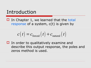
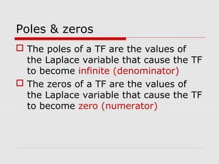
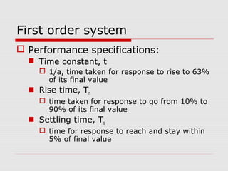
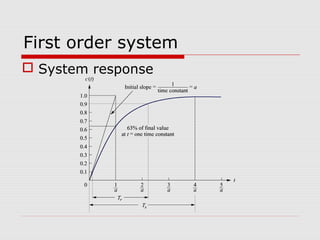
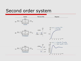
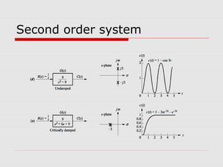
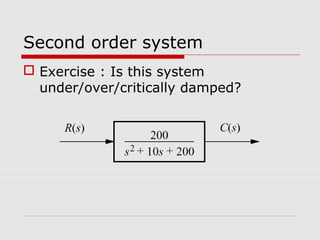
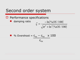
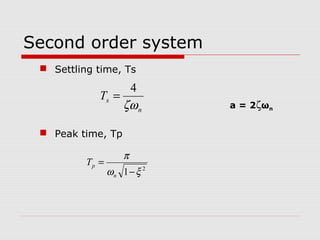
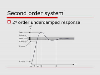
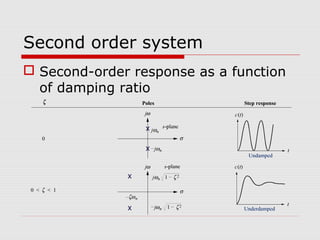
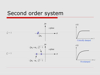
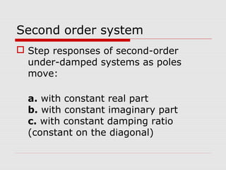
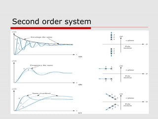
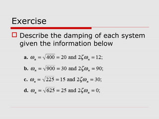
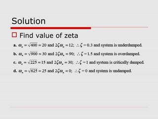
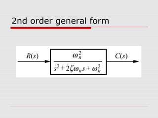
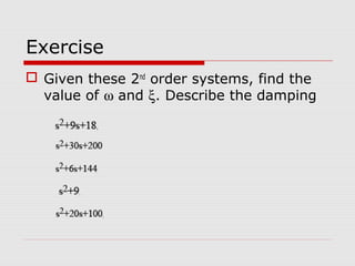
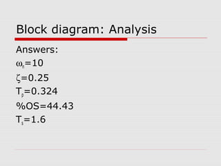
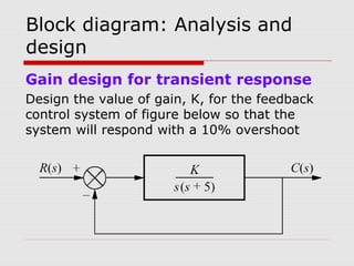
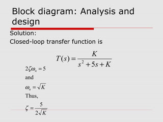
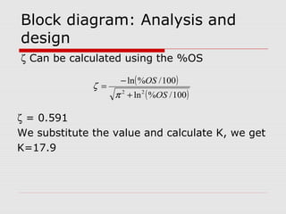
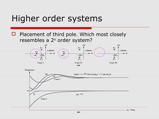
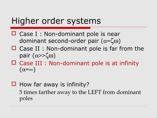
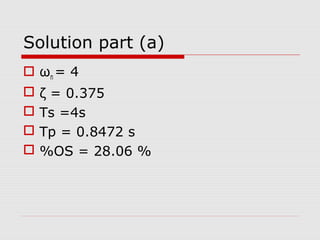
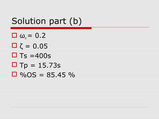
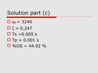
This chapter discusses transient response in control systems. It describes how to determine the time response from a transfer function using poles and zeros. For a first order system, the chapter defines the time constant, rise time and settling time. For a second order system, it defines damping ratio, percent overshoot, settling time and peak time. The chapter also discusses higher order systems and how to approximate them as second order systems. Exercises are provided to analyze systems and design feedback control systems based on desired transient response specifications.

1. CONTROL SYSTEMS THEORY
Transient response
Chapter 4

2. Objectives
 To find time response from transfer
function
 To describe quantitatively the
transient response of a 1st and 2nd
order system
 To determine response of a control
system using poles and zeros

3. Introduction
 In Chapter 1, we learned that the total
response of a system, c(t) is given by
c ( t ) = cforced ( t ) + cnatural ( t )
 In order to qualitatively examine and
describe this output response, the poles and
zeros method is used.

4. Poles & zeros
 The poles of a TF are the values of
the Laplace variable that cause the TF
to become infinite (denominator)
 The zeros of a TF are the values of
the Laplace variable that cause the TF
to become zero (numerator)

5. Poles & zeros
 Example : Given the TF of G(s), find
the poles and zeros
 Solution :
 G(s) = zero/pole
 Pole at s=-5
 Zero at s=-2

6. Poles & zeros
 Zero (o), Pole (x)
 Transfer function = Numerator
Denominator
= Zeros
Poles

7. Poles & zeros
 Example : Given G(s), obtain the
pole-zero plot of the system
Zero (o)
Pole (x)

8. Poles & zeros
 Exercise : Obtain and plot the poles
and zeros for the system given

9. First order system
 First order system with no zeros

10. First order system
 Performance specifications:
 Time constant, t
 1/a, time taken for response to rise to 63%
of its final value
 Rise time, Tr
 time taken for response to go from 10% to
90% of its final value
 Settling time, Ts
 time for response to reach and stay within
5% of final value

11. First order system
 System response

12. Second order system

13. Second order system

14. Second order system
 Exercise : Is this system
under/over/critically damped?

15. Second order system
 Performance specifications
 damping ratio
− ln ( %OS / 100 )
ζ =
π 2 + ln 2 ( %OS / 100 )
 % Overshoot = cmax – cfinal
cfinal
x 100

16. Second order system
 Settling time, Ts
4
Ts =
ζω n
 Peak time, Tp
Tp =
π
ωn 1 − ξ 2
a = 2ζωn

17. Second order system
 2nd order underdamped response

18. Second order system
 Second-order response as a function
of damping ratio

19. Second order system

20. Second order system
 Step responses of second-order
under-damped systems as poles
move:
a. with constant real part
b. with constant imaginary part
c. with constant damping ratio
(constant on the diagonal)

21. Second order system

22. Exercise
 Describe the damping of each system
given the information below

23. Solution
 Find value of zeta

24. 2nd order general form

25. Exercise
 Given these 2nd order systems, find the
value of ω and ξ. Describe the damping

26. Solution

27. Example
 Given
 Find settling time, peak time, %OS
 Hint :

28. Solution

29. Block diagram: Analysis
Finding transient response
For the system shown below, find the
peak time, percent overshoot and
settling time.

30. Block diagram: Analysis
Answers:
ωn=10
ζ=0.25
Tp=0.324
%OS=44.43
Ts=1.6

31. Block diagram: Analysis and
design
Gain design for transient response
Design the value of gain, K, for the feedback
control system of figure below so that the
system will respond with a 10% overshoot

32. Block diagram: Analysis and
design
Solution:
Closed-loop transfer function is
2ζω n = 5
and
ωn = K
Thus,
5
ζ =
2 K
K
T (s) = 2
s + 5s + K

33. Block diagram: Analysis and
design
ζ Can be calculated using the %OS
ζ =
− ln ( %OS / 100 )
π 2 + ln 2 ( %OS / 100 )
ζ = 0.591
We substitute the value and calculate K, we get
K=17.9

34. Higher order systems
 Systems with >2 poles and zeros can
be approximated to 2nd order system
with 2 dominant poles

35. Higher order systems
 Placement of third pole. Which most closely
resembles a 2nd order system?

36. Higher order systems
 Case I : Non-dominant pole is near
dominant second-order pair (α=ζω)
 Case II : Non-dominant pole is far from the
pair (α>>ζω)
 Case III : Non-dominant pole is at infinity
(α=∞)
 How far away is infinity?
5 times farther away to the LEFT from dominant
poles

37. Exercises
 Find ζ, ωn, Ts, Tp and %OS
a)
T(s) =
b) T(s) =
16
s2 + 3s + 16
0.04
s2 + 0.02s + 0.04
c) T(s) =
1.05 x 107
s2 + (1.6 x 103)s + (1.5 x 107)

38. Solution part (a)
 ωn = 4




ζ = 0.375
Ts =4s
Tp = 0.8472 s
%OS = 28.06 %

39. Solution part (b)
 ωn = 0.2




ζ = 0.05
Ts =400s
Tp = 15.73s
%OS = 85.45 %

40. Solution part (c)
 ωn = 3240




ζ = 0.247
Ts =0.005 s
Tp = 0.001 s
%OS = 44.92 %