SlideShare a Scribd company logo
1 of 87
Time Domain Analysis
Introduction
• In time-domain analysis the response of a dynamic system to an input is expressed as a
function of time.
• It is possible to compute the time response of a system if the nature of input and the
mathematical model of the system are known.
• Usually, the input signals to control systems are not known fully ahead of time.
• It is therefore difficult to express the actual input signals mathematically by simple
equations.
Standard Test Signals
• The characteristics of actual input signals are a sudden shock,
a sudden change, a constant velocity, and constant
acceleration.
• The dynamic behavior of a system is therefore judged and
compared under application of standard test signals – an
impulse, a step, a constant velocity, and constant acceleration.
• The other standard signal of great importance is a sinusoidal
signal.
Standard Test Signals
• Impulse signal
– The impulse signal imitate the
sudden shock characteristic of
actual input signal.
– If A=1, the impulse signal is
called unit impulse signal.
0 t
δ(t)
A






00
0
t
tA
t)(
Standard Test Signals
• Step signal
– The step signal imitate
the sudden change
characteristic of actual
input signal.
– If A=1, the step signal is
called unit step signal






00
0
t
tA
tu )( 0 t
u(t)
A
Standard Test Signals
• Ramp signal
– The ramp signal imitate
the constant velocity
characteristic of actual
input signal.
– If A=1, the ramp signal
is called unit ramp
signal






00
0
t
tAt
tr )(
0 t
r(t)
r(t)
unit ramp signal
r(t)
ramp signal with slope A
Standard Test Signals
• Parabolic signal
– The parabolic signal
imitate the constant
acceleration characteristic
of actual input signal.
– If A=1, the parabolic
signal is called unit
parabolic signal.








00
0
2
2
t
t
At
tp )(
0 t
p(t)
parabolic signal with slope A
p(t)
Unit parabolic signal
p(t)
Relation between standard Test Signals
• Impulse
• Step
• Ramp
• Parabolic






00
0
t
tA
t)(






00
0
t
tA
tu )(






00
0
t
tAt
tr )(








00
0
2
2
t
t
At
tp )(


 dt
d
dt
d
dt
d
Laplace Transform of Test Signals
• Impulse
• Step






00
0
t
tA
t)(
AstL  )()}({ 






00
0
t
tA
tu )(
S
A
sUtuL  )()}({
Laplace Transform of Test Signalst
• Ramp
• Parabolic
2
s
A
sRtrL  )()}({
3
)()}({
S
A
sPtpL 






00
0
t
tAt
tr )(








00
0
2
2
t
t
At
tp )(
Time Response of Control Systems
System
• The time response of any system has two components
• Transient response
• Steady-state response.
• Time response of a dynamic system response to an input
expressed as a function of time.
Time Response of Control Systems
• When the response of the system is changed from equilibrium it
takes some time to settle down.
• This is called transient response.
0 2 4 6 8 10 12 14 16 18 20
0
1
2
3
4
5
6
x 10
-3
Step Response
Time (sec)
Amplitude
Response
Step Input
Transient Response
SteadyStateResponse
• The response of the
system after the transient
response is called steady
state response.
Time Response of Control Systems
• Transient response depend upon the system poles only and not
on the type of input.
• It is therefore sufficient to analyze the transient response using a
step input.
• The steady-state response depends on system dynamics and the
input quantity.
• It is then examined using different test signals by final value
theorem.
Introduction
• The first order system has only one pole.
• Where K is the D.C gain and T is the time constant
of the system.
• Time constant is a measure of how quickly a 1st
order system responds to a unit step input.
• D.C Gain of the system is ratio between the input
signal and the steady state value of output.
1

Ts
K
sR
sC
)(
)(
Introduction
• The first order system given below.
13
10


s
sG )(
5
3


s
sG )(
151
53


s/
/
• D.C gain is 10 and time constant is 3 seconds.
• For the following system
• D.C Gain of the system is 3/5 and time constant is 1/5
seconds.
Impulse Response of 1st Order System
• Consider the following 1st order system
1Ts
K
)(sC)(sR
0
t
δ(t)
1
1 )()( ssR 
1

Ts
K
sC )(
Impulse Response of 1st Order System
• Re-arrange following equation as
1

Ts
K
sC )(
Ts
TK
sC
/
/
)(
1

Tt
e
T
K
tc /
)( 

• In order to compute the response of the system in time domain
we need to compute inverse Laplace transform of the above
equation.
at
Ce
as
C
L 







1
Impulse Response of 1st Order System
Tt
e
T
K
tc /
)( 
• If K=3 and T=2s then
0 2 4 6 8 10
0
0.5
1
1.5
Time
c(t)
K/T*exp(-t/T)
Step Response of 1st Order System
• Consider the following 1st order system
1Ts
K
)(sC)(sR
s
sUsR
1
 )()(
 1

Tss
K
sC )(
1

Ts
KT
s
K
sC )(
• In order to find out the inverse Laplace of the above equation, we
need to break it into partial fraction expansion (page 867 in the
Textbook)
Step Response of 1st Order System
• Taking Inverse Laplace of above equation








1
1
Ts
T
s
KsC )(
 Tt
etuKtc /
)()( 

• Where u(t)=1
 Tt
eKtc /
)( 
 1
  KeKtc 63201 1
.)(  
• When t=T (time constant)
Step Response of 1st Order System
• If K=10 and T=1.5s then  Tt
eKtc /
)( 
 1
0 1 2 3 4 5 6 7 8 9 10
0
1
2
3
4
5
6
7
8
9
10
11
Time
c(t)
K*(1-exp(-t/T))
Unit Step Input
Step Response
1
10

Input
outputstatesteady
KGainCD.
%63
Step Response of 1st order System
• System takes five time constants to reach its
final value.
Step Response of 1st Order System
• If K=10 and T=1, 3, 5, 7  Tt
eKtc /
)( 
 1
0 5 10 15
0
1
2
3
4
5
6
7
8
9
10
11
Time
c(t)
K*(1-exp(-t/T))
T=3s
T=5s
T=7s
T=1s
Step Response of 1st Order System
• If K=1, 3, 5, 10 and T=1  Tt
eKtc /
)( 
 1
0 5 10 15
0
1
2
3
4
5
6
7
8
9
10
11
Time
c(t)
K*(1-exp(-t/T))
K=1
K=3
K=5
K=10
Relation Between Step and impulse
response
• The step response of the first order system is
• Differentiating c(t) with respect to t yields
  TtTt
KeKeKtc //
)( 
 1
 Tt
KeK
dt
d
dt
tdc /)( 

Tt
e
T
K
dt
tdc /)( 

Analysis of Simple RC Circuit
)()(
)(
)())((
)(
)()()(
tvtv
dt
tdv
RC
dt
tdv
C
dt
tCvd
ti
tvtvtiR
T
T



state
variable
Input
waveform
±
v(t)C
R
vT(t)
i(t)
Analysis of Simple RC Circuit
Step-input response:
match initial state:
output response for step-input:
v0
v0u(t)
v0(1-e-t/RC)u(t)
)()(
)(
0 tuvtv
dt
tdv
RC 
)()( 0 tuvKetv RC
t


)()1()( 0 tuevtv RC
t

00)(0)0( 00  vKtuvKv
RC Circuit
• v(t) = v0(1 - e-t/RC) -- waveform
under step input v0u(t)
• v(t)=0.5v0  t = 0.69RC
– i.e., delay = 0.69RC (50% delay)
v(t)=0.1v0  t = 0.1RC
v(t)=0.9v0  t = 2.3RC
– i.e., rise time = 2.2RC (if defined as time from 10% to 90% of Vdd)
• For simplicity, industry uses
TD = RC (= Elmore delay)
Elmore Delay
Delay
1. 50%-50%
point delay
2. Delay=0.69
RC
Example 1
• Impulse response of a 1st order system is given below.
• Find out
– Time constant T
– D.C Gain K
– Transfer Function
– Step Response
t
etc 50
3 .
)( 

Example 1
• The Laplace Transform of Impulse response of a
system is actually the transfer function of the system.
• Therefore taking Laplace Transform of the impulse
response given by following equation.
t
etc 50
3 .
)( 

)(
..
)( s
SS
sC 




50
3
1
50
3
50
3
.)(
)(
)(
)(


SsR
sC
s
sC

12
6


SsR
sC
)(
)(
Example 1
• Impulse response of a 1st order system is given below.
• Find out
– Time constant T=2
– D.C Gain K=6
– Transfer Function
– Step Response
t
etc 50
3 .
)( 

12
6


SsR
sC
)(
)(
Example 1
• For step response integrate impulse response
t
etc 50
3 .
)( 

dtedttc t

 50
3 .
)(
Cetc t
s   50
6 .
)(
• We can find out C if initial condition is known e.g. cs(0)=0
Ce   050
60 .
6C
t
s etc 50
66 .
)( 

Example 1
• If initial conditions are not known then partial fraction
expansion is a better choice
12
6


SsR
sC
)(
)(
 12
6


Ss
sC )(
  1212
6


 s
B
s
A
Ss
s
sRsR
1
)(,)( inputstepaissince
  50
66
12
6
.

 ssSs
t
etc 50
66 .
)( 

Ramp Response of 1st Order System
• Consider the following 1st order system
1Ts
K
)(sC)(sR
2
1
s
sR )(
 12


Tss
K
sC )(
• The ramp response is given as
 Tt
TeTtKtc /
)( 

Parabolic Response of 1st Order System
• Consider the following 1st order system
1Ts
K
)(sC)(sR
3
1
s
sR )(
 13


Tss
K
sC )(Therefore,
Practical Determination of Transfer
Function of 1st Order Systems
• Often it is not possible or practical to obtain a system's
transfer function analytically.
• Perhaps the system is closed, and the component parts are
not easily identifiable.
• The system's step response can lead to a representation even
though the inner construction is not known.
• With a step input, we can measure the time constant and the
steady-state value, from which the transfer function can be
calculated.
Practical Determination of Transfer
Function of 1st Order Systems
• If we can identify T and K empirically we can obtain the
transfer function of the system.
1

Ts
K
sR
sC
)(
)(
Practical Determination of Transfer Function
of 1st Order Systems
• For example, assume the unit
step response given in figure.
• From the response, we can
measure the time constant, that
is, the time for the amplitude to
reach 63% of its final value.
• Since the final value is about
0.72 the time constant is
evaluated where the curve
reaches 0.63 x 0.72 = 0.45, or
about 0.13 second.
T=0.13s
K=0.72
• K is simply steady state value.
• Thus transfer function is
obtained as:
77
55
1130
720
.
.
.
.
)(
)(




sssR
sC
First Order System with a Zero
• Zero of the system lie at -1/α and pole at -1/T.
1
1



Ts
sK
sR
sC )(
)(
)( 
 1
1



Tss
sK
sC
)(
)(

• Step response of the system would be:
 1


Ts
TK
s
K
sC
)(
)(

Tt
eT
T
K
Ktc /
)()( 
 
First Order System With Delays
• Following transfer function is the generic
representation of 1st order system with time
lag.
• Where td is the delay time.
dst
e
Ts
K
sR
sC 


1)(
)(
First Order System With Delays
dst
e
Ts
K
sR
sC 


1)(
)(
1
Unit Step
Step Response
t
td
First Order System With Delays
)2(]10)2(10[
])
3/1
1010
[(
)()()]([
)13(
10
)(
13
10
)(
)(
)2(3/1
21
1
2
2















tuet
e
ss
L
tutfsFeL
e
ss
sC
e
ssR
sC
t
s
s
s
s
0 5 10 15
0
2
4
6
8
10
Step Response
Time (sec)
Amplitude
std 2
sT 3
10K
Second Order System
• We have already discussed the affect of location of poles and zeros on
the transient response of 1st order systems.
• Compared to the simplicity of a first-order system, a second-order system
exhibits a wide range of responses that must be analyzed and described.
• Varying a first-order system's parameter (T, K) simply changes the speed
and offset of the response
• Whereas, changes in the parameters of a second-order system can
change the form of the response.
• A second-order system can display characteristics much like a first-order
system or, depending on component values, display damped or pure
oscillations for its transient response. 44
Introduction
• A general second-order system is characterized by the
following transfer function.
22
2
2 nn
n
sssR
sC




)(
)(
45
un-damped natural frequency of the second order system,
which is the frequency of oscillation of the system without
damping.
n
damping ratio of the second order system, which is a measure
of the degree of resistance to change in the system output.

Example 2
42
4
2


sssR
sC
)(
)(
• Determine the un-damped natural frequency and damping ratio
of the following second order system.
42
n
22
2
2 nn
n
sssR
sC




)(
)(
• Compare the numerator and denominator of the given transfer
function with the general 2nd order transfer function.
2 n ssn 22  
422 222
 ssss nn 
50. 
1 n
46
Introduction
22
2
2 nn
n
sssR
sC




)(
)(
• Two poles of the system are
1
1
2
2




nn
nn
47
Introduction
• According the value of , a second-order system can be set into
one of the four categories (page 169 in the textbook):
1
1
2
2




nn
nn

1. Overdamped - when the system has two real distinct poles ( >1).
-a-b-c
δ
jω
48
Introduction
• According the value of , a second-order system can be set into
one of the four categories (page 169 in the textbook):
1
1
2
2




nn
nn

2. Underdamped - when the system has two complex conjugate poles (0 < <1)
-a-b-c
δ
jω
49
Introduction
• According the value of , a second-order system can be set into
one of the four categories (page 169 in the textbook):
1
1
2
2




nn
nn

3. Undamped - when the system has two imaginary poles ( = 0).
-a-b-c
δ
jω
50
Introduction
• According the value of , a second-order system can be set into
one of the four categories (page 169 in the textbook):
1
1
2
2




nn
nn

4. Critically damped - when the system has two real but equal poles ( = 1).
-a-b-c
δ
jω
51
Underdamped System
52
For 0< <1 and ωn > 0, the 2nd order system’s response due to a
unit step input is as follows.
Important timing characteristics: delay time, rise time, peak
time, maximum overshoot, and settling time.

Delay Time
53
• The delay (td) time is the time required for the response to
reach half the final value the very first time.
Rise Time
• The rise time is the time required for the response to rise from 10%
to 90%, 5% to 95%, or 0% to 100% of its final value.
• For underdamped second order systems, the 0% to 100% rise time is
normally used. For overdamped systems, the 10% to 90% rise time is
commonly used.
Peak Time
55
• The peak time is the time required for the response to reach
the first peak of the overshoot.
5555
Maximum Overshoot
56
The maximum overshoot is the maximum peak value of the
response curve measured from unity. If the final steady-state
value of the response differs from unity, then it is common to
use the maximum percent overshoot. It is defined by
The amount of the maximum (percent) overshoot directly
indicates the relative stability of the system.
Settling Time
57
• The settling time is the time required for the response curve
to reach and stay within a range about the final value of size
specified by absolute percentage of the final value (usually 2%
or 5%).
Step Response of underdamped System
222222
2
21
nnnn
n
ss
s
s
sC




)(
• The partial fraction expansion of above equation is given as
22
2
21
nn
n
ss
s
s
sC




)(
 2
2 ns 
 22
1  n
   222
1
21





nn
n
s
s
s
sC )(
22
2
2 nn
n
sssR
sC




)(
)(
 22
2
2 nn
n
sss
sC



)(
Step Response
58
Step Response of underdamped System
• Above equation can be written as
   222
1
21





nn
n
s
s
s
sC )(
  22
21
dn
n
s
s
s
sC




)(
2
1   nd• Where , is the frequency of transient oscillations
and is called damped natural frequency.
• The inverse Laplace transform of above equation can be obtained
easily if C(s) is written in the following form:
    2222
1
dn
n
dn
n
ss
s
s
sC








)(
59
Step Response of underdamped System
    2222
1
dn
n
dn
n
ss
s
s
sC








)(
    22
2
2
22
1
11
dn
n
dn
n
ss
s
s
sC












)(
    22222
1
1
dn
d
dn
n
ss
s
s
sC










)(
tetetc d
t
d
t nn



 
sincos)( 


2
1
1
60
Step Response of underdamped System
tetetc d
t
d
t nn



 
sincos)( 


2
1
1









 
ttetc dd
tn




sincos)(
2
1
1
n
nd



 2
1
• When 0
ttc ncos)(  1
61
Step Response of underdamped System









 
ttetc dd
tn




sincos)(
2
1
1
3and1.0if  n
0 2 4 6 8 10
0
0.2
0.4
0.6
0.8
1
1.2
1.4
1.6
1.8
62
Step Response of underdamped System









 
ttetc dd
tn




sincos)(
2
1
1
3and5.0if  n
0 2 4 6 8 10
0
0.2
0.4
0.6
0.8
1
1.2
1.4
63
Step Response of underdamped System









 
ttetc dd
tn




sincos)(
2
1
1
3and9.0if  n
0 2 4 6 8 10
0
0.2
0.4
0.6
0.8
1
1.2
1.4
64
Step Response of underdamped System









 
ttetc dd
tn




sincos)(
2
1
1
65
S-Plane (Underdamped System)

1
1
2
2




nn
nn
66
Since 𝜔2 𝜁2 − 𝜔2 𝜁2 − 1 = 𝜔2, the distance
from the pole to the origin is 𝜔 and 𝜁 = 𝑐𝑜𝑠𝛽
Analytical Solution
• Page 171 in the textbook
• Rise time: set c(t)=1, we have 𝑡 𝑟 =
𝜋−𝛽
𝜔 𝑑
• Peak time: set
𝑑𝑐(𝑡)
𝑑𝑡
= 0, we have 𝑡 𝑝 =
𝜋
𝜔 𝑑
• Maximum overshoot: M 𝑝 = 𝑐 𝑡 𝑝 − 1 =
𝑒−(𝜁𝜔/𝜔 𝑑)𝜋
(for unity output)
• Settling time: the time for the outputs always
within 2% of the final value is approximately
4
𝜁𝜔









 
ttetc dd
tn




sincos)(
2
1
1
2
1   nd
Empirical Solution Using MATLAB
• Page 242 in the textbook
Steady State Error
• If the output of a control system at steady state does not
exactly match with the input, the system is said to have
steady state error
• Any physical control system inherently suffers steady-state
error in response to certain types of inputs.
• Page 219 in the textbook
• A system may have no steady-state error to a step input, but
the same system may exhibit nonzero steady-state error to a
ramp input.
Classification of Control Systems
• Control systems may be classified according to
their ability to follow step inputs, ramp inputs,
parabolic inputs, and so on.
• The magnitudes of the steady-state errors due
to these individual inputs are indicative of the
goodness of the system.
Classification of Control Systems
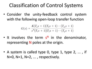
• Consider the unity-feedback control system
with the following open-loop transfer function
• It involves the term sN in the denominator,
representing N poles at the origin.
• A system is called type 0, type 1, type 2, ... , if
N=0, N=1, N=2, ... , respectively.
Classification of Control Systems
• As the type number is increased, accuracy is
improved.
• However, increasing the type number
aggravates the stability problem.
• A compromise between steady-state accuracy
and relative stability is always necessary.
Steady State Error of Unity Feedback Systems
• Consider the system shown in following figure.
• The closed-loop transfer function is
Steady State Error of Unity Feedback Systems
• The transfer function between the error signal E(s) and the
input signal R(s) is
)()(
)(
sGsR
sE


1
1
• The final-value theorem provides a convenient way to find
the steady-state performance of a stable system.
• Since E(s) is
• The steady state error is
• Steady state error is defined as the error between the
input signal and the output signal when 𝑡 → ∞.
Static Error Constants
• The static error constants are figures of merit of
control systems. The higher the constants, the
smaller the steady-state error.
• In a given system, the output may be the position,
velocity, pressure, temperature, or the like.
• Therefore, in what follows, we shall call the output
“position,” the rate of change of the output
“velocity,” and so on.
• This means that in a temperature control system
“position” represents the output temperature,
“velocity” represents the rate of change of the
output temperature, and so on.
Static Position Error Constant (Kp)
• The steady-state error of the system for a unit-step input is
• The static position error constant Kp is defined by
• Thus, the steady-state error in terms of the static position
error constant Kp is given by
Static Position Error Constant (Kp)
• For a Type 0 system
• For Type 1 or higher order systems
• For a unit step input the steady state error ess is
• The steady-state error of the system for a unit-ramp input is
• The static velocity error constant Kv is defined by
• Thus, the steady-state error in terms of the static velocity
error constant Kv is given by
Static Velocity Error Constant (Kv)
• For a Type 0 system
• For Type 1 systems
• For type 2 or higher order systems
Static Velocity Error Constant (Kv)
• For a ramp input the steady state error ess is
• The steady-state error of the system for parabolic input is
• The static acceleration error constant Ka is defined by
• Thus, the steady-state error in terms of the static acceleration
error constant Ka is given by
Static Acceleration Error Constant (Ka)
• For a Type 0 system
• For Type 1 systems
• For type 2 systems
• For type 3 or higher order systems
Static Acceleration Error Constant (Ka)
• For a parabolic input the steady state error ess is
Summary
Example 2
• For the system shown in figure below evaluate the static
error constants and find the expected steady state errors
for the standard step, ramp and parabolic inputs.
C(S)R(S) -
))((
))((
128
52100
2


sss
ss
Example 2
))((
))((
)(
128
52100
2



sss
ss
sG
)(lim sGK
s
p
0










 ))((
))((
lim
128
52100
2
0 sss
ss
K
s
p
pK
)(lim ssGK
s
v
0










 ))((
))((
lim
128
52100
2
0 sss
sss
K
s
v
vK
)(lim sGsK
s
a
2
0












 ))((
))((
lim
128
52100
2
2
0 sss
sss
K
s
a
410
12080
5020100
.
))((
))((








aK
Example 2
pK vK 410.aK
0
0
090.

More Related Content

What's hot

Meeting w3 chapter 2 part 1
Meeting w3   chapter 2 part 1Meeting w3   chapter 2 part 1
Meeting w3 chapter 2 part 1mkazree
 
Chapter 4 time domain analysis
Chapter 4 time domain analysisChapter 4 time domain analysis
Chapter 4 time domain analysisBin Biny Bino
 
Lecture 2 transfer-function
Lecture 2 transfer-functionLecture 2 transfer-function
Lecture 2 transfer-functionSaifullah Memon
 
Lecture 13 14-time_domain_analysis_of_1st_order_systems
Lecture 13 14-time_domain_analysis_of_1st_order_systemsLecture 13 14-time_domain_analysis_of_1st_order_systems
Lecture 13 14-time_domain_analysis_of_1st_order_systemsSaifullah Memon
 
ppt on Time Domain and Frequency Domain Analysis
ppt on Time Domain and Frequency Domain Analysisppt on Time Domain and Frequency Domain Analysis
ppt on Time Domain and Frequency Domain Analysissagar_kamble
 
Control system basics, block diagram and signal flow graph
Control system basics, block diagram and signal flow graphControl system basics, block diagram and signal flow graph
Control system basics, block diagram and signal flow graphSHARMA NAVEEN
 
State space analysis.pptx
State space analysis.pptxState space analysis.pptx
State space analysis.pptxRaviMuthamala1
 
Modern Control - Lec07 - State Space Modeling of LTI Systems
Modern Control - Lec07 - State Space Modeling of LTI SystemsModern Control - Lec07 - State Space Modeling of LTI Systems
Modern Control - Lec07 - State Space Modeling of LTI SystemsAmr E. Mohamed
 
Time response analysis
Time response analysisTime response analysis
Time response analysisKaushal Patel
 
Dcs lec03 - z-analysis of discrete time control systems
Dcs   lec03 - z-analysis of discrete time control systemsDcs   lec03 - z-analysis of discrete time control systems
Dcs lec03 - z-analysis of discrete time control systemsAmr E. Mohamed
 
TIME RESPONSE ANALYSIS
TIME RESPONSE ANALYSISTIME RESPONSE ANALYSIS
TIME RESPONSE ANALYSISDeep Chaudhari
 
Discrete state space model 9th &10th lecture
Discrete  state space model   9th  &10th  lectureDiscrete  state space model   9th  &10th  lecture
Discrete state space model 9th &10th lectureKhalaf Gaeid Alshammery
 
Modern Control - Lec 03 - Feedback Control Systems Performance and Characteri...
Modern Control - Lec 03 - Feedback Control Systems Performance and Characteri...Modern Control - Lec 03 - Feedback Control Systems Performance and Characteri...
Modern Control - Lec 03 - Feedback Control Systems Performance and Characteri...Amr E. Mohamed
 
Root locus method
Root locus methodRoot locus method
Root locus methodRavi Patel
 
STate Space Analysis
STate Space AnalysisSTate Space Analysis
STate Space AnalysisHussain K
 
Control system stability routh hurwitz criterion
Control system stability routh hurwitz criterionControl system stability routh hurwitz criterion
Control system stability routh hurwitz criterionNilesh Bhaskarrao Bahadure
 
Lecture 6 modelling-of_electrical__electronic_systems
Lecture 6 modelling-of_electrical__electronic_systemsLecture 6 modelling-of_electrical__electronic_systems
Lecture 6 modelling-of_electrical__electronic_systemsSaifullah Memon
 
Control systems engineering
Control systems engineeringControl systems engineering
Control systems engineeringAnisur Rahman
 

What's hot (20)

Meeting w3 chapter 2 part 1
Meeting w3   chapter 2 part 1Meeting w3   chapter 2 part 1
Meeting w3 chapter 2 part 1
 
Chapter 4 time domain analysis
Chapter 4 time domain analysisChapter 4 time domain analysis
Chapter 4 time domain analysis
 
Lecture 2 transfer-function
Lecture 2 transfer-functionLecture 2 transfer-function
Lecture 2 transfer-function
 
Lecture 13 14-time_domain_analysis_of_1st_order_systems
Lecture 13 14-time_domain_analysis_of_1st_order_systemsLecture 13 14-time_domain_analysis_of_1st_order_systems
Lecture 13 14-time_domain_analysis_of_1st_order_systems
 
ppt on Time Domain and Frequency Domain Analysis
ppt on Time Domain and Frequency Domain Analysisppt on Time Domain and Frequency Domain Analysis
ppt on Time Domain and Frequency Domain Analysis
 
Control system basics, block diagram and signal flow graph
Control system basics, block diagram and signal flow graphControl system basics, block diagram and signal flow graph
Control system basics, block diagram and signal flow graph
 
State space analysis.pptx
State space analysis.pptxState space analysis.pptx
State space analysis.pptx
 
Modern Control - Lec07 - State Space Modeling of LTI Systems
Modern Control - Lec07 - State Space Modeling of LTI SystemsModern Control - Lec07 - State Space Modeling of LTI Systems
Modern Control - Lec07 - State Space Modeling of LTI Systems
 
Time response analysis
Time response analysisTime response analysis
Time response analysis
 
Dcs lec03 - z-analysis of discrete time control systems
Dcs   lec03 - z-analysis of discrete time control systemsDcs   lec03 - z-analysis of discrete time control systems
Dcs lec03 - z-analysis of discrete time control systems
 
Root locus
Root locus Root locus
Root locus
 
TIME RESPONSE ANALYSIS
TIME RESPONSE ANALYSISTIME RESPONSE ANALYSIS
TIME RESPONSE ANALYSIS
 
Discrete state space model 9th &10th lecture
Discrete  state space model   9th  &10th  lectureDiscrete  state space model   9th  &10th  lecture
Discrete state space model 9th &10th lecture
 
Modern Control - Lec 03 - Feedback Control Systems Performance and Characteri...
Modern Control - Lec 03 - Feedback Control Systems Performance and Characteri...Modern Control - Lec 03 - Feedback Control Systems Performance and Characteri...
Modern Control - Lec 03 - Feedback Control Systems Performance and Characteri...
 
Root locus method
Root locus methodRoot locus method
Root locus method
 
6. steady state error
6. steady state error6. steady state error
6. steady state error
 
STate Space Analysis
STate Space AnalysisSTate Space Analysis
STate Space Analysis
 
Control system stability routh hurwitz criterion
Control system stability routh hurwitz criterionControl system stability routh hurwitz criterion
Control system stability routh hurwitz criterion
 
Lecture 6 modelling-of_electrical__electronic_systems
Lecture 6 modelling-of_electrical__electronic_systemsLecture 6 modelling-of_electrical__electronic_systems
Lecture 6 modelling-of_electrical__electronic_systems
 
Control systems engineering
Control systems engineeringControl systems engineering
Control systems engineering
 

Similar to Time domain analysis

time domain analysis.pptx
time domain analysis.pptxtime domain analysis.pptx
time domain analysis.pptxdeepaMS4
 
Time domain analysis
Time domain analysisTime domain analysis
Time domain analysisHussain K
 
LCE-UNIT 1 PPT.pdf
LCE-UNIT 1 PPT.pdfLCE-UNIT 1 PPT.pdf
LCE-UNIT 1 PPT.pdfHODECE21
 
Order of instruments.ppt
Order of instruments.pptOrder of instruments.ppt
Order of instruments.pptANURUPAa
 
lecture1 (5).ppt
lecture1 (5).pptlecture1 (5).ppt
lecture1 (5).pptHebaEng
 
Lecture 13 14-time_domain_analysis_of_1st_order_systems
Lecture 13 14-time_domain_analysis_of_1st_order_systemsLecture 13 14-time_domain_analysis_of_1st_order_systems
Lecture 13 14-time_domain_analysis_of_1st_order_systemsSALEH846
 
Time response and analysis kaushal shah
Time response and analysis kaushal shahTime response and analysis kaushal shah
Time response and analysis kaushal shahKaushal Shah
 
Chapter 3-Dynamic Behavior of First and Second Order Processes-1.pptx
Chapter 3-Dynamic Behavior of First and Second Order Processes-1.pptxChapter 3-Dynamic Behavior of First and Second Order Processes-1.pptx
Chapter 3-Dynamic Behavior of First and Second Order Processes-1.pptxaduladube0992
 
time domain analysis, Rise Time, Delay time, Damping Ratio, Overshoot, Settli...
time domain analysis, Rise Time, Delay time, Damping Ratio, Overshoot, Settli...time domain analysis, Rise Time, Delay time, Damping Ratio, Overshoot, Settli...
time domain analysis, Rise Time, Delay time, Damping Ratio, Overshoot, Settli...Waqas Afzal
 
Time response in systems
Time response in systemsTime response in systems
Time response in systemsSatheeshCS2
 
Lecture 12 time_domain_analysis_of_control_systems
Lecture 12 time_domain_analysis_of_control_systemsLecture 12 time_domain_analysis_of_control_systems
Lecture 12 time_domain_analysis_of_control_systemsSaifullah Memon
 
Time domain definition 6
Time domain definition 6Time domain definition 6
Time domain definition 6Syed Saeed
 
Time domain definition 6
Time domain definition 6Time domain definition 6
Time domain definition 6Syed Saeed
 
CONTROL SYSTEM SOURAV MONDAL.pptx
CONTROL SYSTEM SOURAV MONDAL.pptxCONTROL SYSTEM SOURAV MONDAL.pptx
CONTROL SYSTEM SOURAV MONDAL.pptxSouravMondal831575
 
Time domain definition 6
Time domain definition 6Time domain definition 6
Time domain definition 6Syed Saeed
 
Definition classification
Definition classificationDefinition classification
Definition classificationSyed Saeed
 

Similar to Time domain analysis (20)

time domain analysis.pptx
time domain analysis.pptxtime domain analysis.pptx
time domain analysis.pptx
 
Time domain analysis
Time domain analysisTime domain analysis
Time domain analysis
 
LCE-UNIT 1 PPT.pdf
LCE-UNIT 1 PPT.pdfLCE-UNIT 1 PPT.pdf
LCE-UNIT 1 PPT.pdf
 
time response analysis
time response analysistime response analysis
time response analysis
 
Order of instruments.ppt
Order of instruments.pptOrder of instruments.ppt
Order of instruments.ppt
 
lecture1 (5).ppt
lecture1 (5).pptlecture1 (5).ppt
lecture1 (5).ppt
 
Lecture 13 14-time_domain_analysis_of_1st_order_systems
Lecture 13 14-time_domain_analysis_of_1st_order_systemsLecture 13 14-time_domain_analysis_of_1st_order_systems
Lecture 13 14-time_domain_analysis_of_1st_order_systems
 
Csl9 4 f15
Csl9 4 f15Csl9 4 f15
Csl9 4 f15
 
Time response and analysis kaushal shah
Time response and analysis kaushal shahTime response and analysis kaushal shah
Time response and analysis kaushal shah
 
Chapter 3-Dynamic Behavior of First and Second Order Processes-1.pptx
Chapter 3-Dynamic Behavior of First and Second Order Processes-1.pptxChapter 3-Dynamic Behavior of First and Second Order Processes-1.pptx
Chapter 3-Dynamic Behavior of First and Second Order Processes-1.pptx
 
03 dynamic.system.
03 dynamic.system.03 dynamic.system.
03 dynamic.system.
 
time domain analysis, Rise Time, Delay time, Damping Ratio, Overshoot, Settli...
time domain analysis, Rise Time, Delay time, Damping Ratio, Overshoot, Settli...time domain analysis, Rise Time, Delay time, Damping Ratio, Overshoot, Settli...
time domain analysis, Rise Time, Delay time, Damping Ratio, Overshoot, Settli...
 
Time response in systems
Time response in systemsTime response in systems
Time response in systems
 
Lecture 12 time_domain_analysis_of_control_systems
Lecture 12 time_domain_analysis_of_control_systemsLecture 12 time_domain_analysis_of_control_systems
Lecture 12 time_domain_analysis_of_control_systems
 
Time domain definition 6
Time domain definition 6Time domain definition 6
Time domain definition 6
 
Time domain definition 6
Time domain definition 6Time domain definition 6
Time domain definition 6
 
Me314 week 06-07-Time Response
Me314 week 06-07-Time ResponseMe314 week 06-07-Time Response
Me314 week 06-07-Time Response
 
CONTROL SYSTEM SOURAV MONDAL.pptx
CONTROL SYSTEM SOURAV MONDAL.pptxCONTROL SYSTEM SOURAV MONDAL.pptx
CONTROL SYSTEM SOURAV MONDAL.pptx
 
Time domain definition 6
Time domain definition 6Time domain definition 6
Time domain definition 6
 
Definition classification
Definition classificationDefinition classification
Definition classification
 

More from Mohammed Waris Senan (20)

Basics of rotating machines
Basics of rotating machinesBasics of rotating machines
Basics of rotating machines
 
Introduction to Integral calculus
Introduction to Integral calculusIntroduction to Integral calculus
Introduction to Integral calculus
 
Introduction to Differential calculus
Introduction to Differential calculusIntroduction to Differential calculus
Introduction to Differential calculus
 
Control system unit(1)
Control system unit(1)Control system unit(1)
Control system unit(1)
 
Magnetic materials & B-H Curve
Magnetic materials & B-H CurveMagnetic materials & B-H Curve
Magnetic materials & B-H Curve
 
Measurement of 3 phase power by two watt-meter method
Measurement of 3 phase power by two watt-meter methodMeasurement of 3 phase power by two watt-meter method
Measurement of 3 phase power by two watt-meter method
 
Electrical machine slide share
Electrical machine slide shareElectrical machine slide share
Electrical machine slide share
 
Electromechanical energy conversion
Electromechanical energy conversionElectromechanical energy conversion
Electromechanical energy conversion
 
Dc machines (Generator & Motor)
Dc machines (Generator & Motor)Dc machines (Generator & Motor)
Dc machines (Generator & Motor)
 
Single and three phase Transformers
Single and three phase TransformersSingle and three phase Transformers
Single and three phase Transformers
 
Network synthesis
Network synthesisNetwork synthesis
Network synthesis
 
Two port networks
Two port networksTwo port networks
Two port networks
 
Transient analysis
Transient analysisTransient analysis
Transient analysis
 
Laplace transform
Laplace transformLaplace transform
Laplace transform
 
Active network
Active networkActive network
Active network
 
Transformer
TransformerTransformer
Transformer
 
Synchronous machines
Synchronous machinesSynchronous machines
Synchronous machines
 
Magnetic circuit
Magnetic circuitMagnetic circuit
Magnetic circuit
 
Induction machines
Induction machinesInduction machines
Induction machines
 
Basic
BasicBasic
Basic
 

Recently uploaded

Karra SKD Conference Presentation Revised.pptx
Karra SKD Conference Presentation Revised.pptxKarra SKD Conference Presentation Revised.pptx
Karra SKD Conference Presentation Revised.pptxAshokKarra1
 
call girls in Kamla Market (DELHI) 🔝 >༒9953330565🔝 genuine Escort Service 🔝✔️✔️
call girls in Kamla Market (DELHI) 🔝 >༒9953330565🔝 genuine Escort Service 🔝✔️✔️call girls in Kamla Market (DELHI) 🔝 >༒9953330565🔝 genuine Escort Service 🔝✔️✔️
call girls in Kamla Market (DELHI) 🔝 >༒9953330565🔝 genuine Escort Service 🔝✔️✔️9953056974 Low Rate Call Girls In Saket, Delhi NCR
 
MULTIDISCIPLINRY NATURE OF THE ENVIRONMENTAL STUDIES.pptx
MULTIDISCIPLINRY NATURE OF THE ENVIRONMENTAL STUDIES.pptxMULTIDISCIPLINRY NATURE OF THE ENVIRONMENTAL STUDIES.pptx
MULTIDISCIPLINRY NATURE OF THE ENVIRONMENTAL STUDIES.pptxAnupkumar Sharma
 
Inclusivity Essentials_ Creating Accessible Websites for Nonprofits .pdf
Inclusivity Essentials_ Creating Accessible Websites for Nonprofits .pdfInclusivity Essentials_ Creating Accessible Websites for Nonprofits .pdf
Inclusivity Essentials_ Creating Accessible Websites for Nonprofits .pdfTechSoup
 
INTRODUCTION TO CATHOLIC CHRISTOLOGY.pptx
INTRODUCTION TO CATHOLIC CHRISTOLOGY.pptxINTRODUCTION TO CATHOLIC CHRISTOLOGY.pptx
INTRODUCTION TO CATHOLIC CHRISTOLOGY.pptxHumphrey A Beña
 
ENGLISH 7_Q4_LESSON 2_ Employing a Variety of Strategies for Effective Interp...
ENGLISH 7_Q4_LESSON 2_ Employing a Variety of Strategies for Effective Interp...ENGLISH 7_Q4_LESSON 2_ Employing a Variety of Strategies for Effective Interp...
ENGLISH 7_Q4_LESSON 2_ Employing a Variety of Strategies for Effective Interp...JhezDiaz1
 
Keynote by Prof. Wurzer at Nordex about IP-design
Keynote by Prof. Wurzer at Nordex about IP-designKeynote by Prof. Wurzer at Nordex about IP-design
Keynote by Prof. Wurzer at Nordex about IP-designMIPLM
 
Computed Fields and api Depends in the Odoo 17
Computed Fields and api Depends in the Odoo 17Computed Fields and api Depends in the Odoo 17
Computed Fields and api Depends in the Odoo 17Celine George
 
How to do quick user assign in kanban in Odoo 17 ERP
How to do quick user assign in kanban in Odoo 17 ERPHow to do quick user assign in kanban in Odoo 17 ERP
How to do quick user assign in kanban in Odoo 17 ERPCeline George
 
4.18.24 Movement Legacies, Reflection, and Review.pptx
4.18.24 Movement Legacies, Reflection, and Review.pptx4.18.24 Movement Legacies, Reflection, and Review.pptx
4.18.24 Movement Legacies, Reflection, and Review.pptxmary850239
 
USPS® Forced Meter Migration - How to Know if Your Postage Meter Will Soon be...
USPS® Forced Meter Migration - How to Know if Your Postage Meter Will Soon be...USPS® Forced Meter Migration - How to Know if Your Postage Meter Will Soon be...
USPS® Forced Meter Migration - How to Know if Your Postage Meter Will Soon be...Postal Advocate Inc.
 
Difference Between Search & Browse Methods in Odoo 17
Difference Between Search & Browse Methods in Odoo 17Difference Between Search & Browse Methods in Odoo 17
Difference Between Search & Browse Methods in Odoo 17Celine George
 
Barangay Council for the Protection of Children (BCPC) Orientation.pptx
Barangay Council for the Protection of Children (BCPC) Orientation.pptxBarangay Council for the Protection of Children (BCPC) Orientation.pptx
Barangay Council for the Protection of Children (BCPC) Orientation.pptxCarlos105
 
ACC 2024 Chronicles. Cardiology. Exam.pdf
ACC 2024 Chronicles. Cardiology. Exam.pdfACC 2024 Chronicles. Cardiology. Exam.pdf
ACC 2024 Chronicles. Cardiology. Exam.pdfSpandanaRallapalli
 
ANG SEKTOR NG agrikultura.pptx QUARTER 4
ANG SEKTOR NG agrikultura.pptx QUARTER 4ANG SEKTOR NG agrikultura.pptx QUARTER 4
ANG SEKTOR NG agrikultura.pptx QUARTER 4MiaBumagat1
 
What is Model Inheritance in Odoo 17 ERP
What is Model Inheritance in Odoo 17 ERPWhat is Model Inheritance in Odoo 17 ERP
What is Model Inheritance in Odoo 17 ERPCeline George
 
Judging the Relevance and worth of ideas part 2.pptx
Judging the Relevance  and worth of ideas part 2.pptxJudging the Relevance  and worth of ideas part 2.pptx
Judging the Relevance and worth of ideas part 2.pptxSherlyMaeNeri
 

Recently uploaded (20)

Karra SKD Conference Presentation Revised.pptx
Karra SKD Conference Presentation Revised.pptxKarra SKD Conference Presentation Revised.pptx
Karra SKD Conference Presentation Revised.pptx
 
call girls in Kamla Market (DELHI) 🔝 >༒9953330565🔝 genuine Escort Service 🔝✔️✔️
call girls in Kamla Market (DELHI) 🔝 >༒9953330565🔝 genuine Escort Service 🔝✔️✔️call girls in Kamla Market (DELHI) 🔝 >༒9953330565🔝 genuine Escort Service 🔝✔️✔️
call girls in Kamla Market (DELHI) 🔝 >༒9953330565🔝 genuine Escort Service 🔝✔️✔️
 
MULTIDISCIPLINRY NATURE OF THE ENVIRONMENTAL STUDIES.pptx
MULTIDISCIPLINRY NATURE OF THE ENVIRONMENTAL STUDIES.pptxMULTIDISCIPLINRY NATURE OF THE ENVIRONMENTAL STUDIES.pptx
MULTIDISCIPLINRY NATURE OF THE ENVIRONMENTAL STUDIES.pptx
 
Inclusivity Essentials_ Creating Accessible Websites for Nonprofits .pdf
Inclusivity Essentials_ Creating Accessible Websites for Nonprofits .pdfInclusivity Essentials_ Creating Accessible Websites for Nonprofits .pdf
Inclusivity Essentials_ Creating Accessible Websites for Nonprofits .pdf
 
INTRODUCTION TO CATHOLIC CHRISTOLOGY.pptx
INTRODUCTION TO CATHOLIC CHRISTOLOGY.pptxINTRODUCTION TO CATHOLIC CHRISTOLOGY.pptx
INTRODUCTION TO CATHOLIC CHRISTOLOGY.pptx
 
ENGLISH 7_Q4_LESSON 2_ Employing a Variety of Strategies for Effective Interp...
ENGLISH 7_Q4_LESSON 2_ Employing a Variety of Strategies for Effective Interp...ENGLISH 7_Q4_LESSON 2_ Employing a Variety of Strategies for Effective Interp...
ENGLISH 7_Q4_LESSON 2_ Employing a Variety of Strategies for Effective Interp...
 
Keynote by Prof. Wurzer at Nordex about IP-design
Keynote by Prof. Wurzer at Nordex about IP-designKeynote by Prof. Wurzer at Nordex about IP-design
Keynote by Prof. Wurzer at Nordex about IP-design
 
Computed Fields and api Depends in the Odoo 17
Computed Fields and api Depends in the Odoo 17Computed Fields and api Depends in the Odoo 17
Computed Fields and api Depends in the Odoo 17
 
How to do quick user assign in kanban in Odoo 17 ERP
How to do quick user assign in kanban in Odoo 17 ERPHow to do quick user assign in kanban in Odoo 17 ERP
How to do quick user assign in kanban in Odoo 17 ERP
 
4.18.24 Movement Legacies, Reflection, and Review.pptx
4.18.24 Movement Legacies, Reflection, and Review.pptx4.18.24 Movement Legacies, Reflection, and Review.pptx
4.18.24 Movement Legacies, Reflection, and Review.pptx
 
FINALS_OF_LEFT_ON_C'N_EL_DORADO_2024.pptx
FINALS_OF_LEFT_ON_C'N_EL_DORADO_2024.pptxFINALS_OF_LEFT_ON_C'N_EL_DORADO_2024.pptx
FINALS_OF_LEFT_ON_C'N_EL_DORADO_2024.pptx
 
USPS® Forced Meter Migration - How to Know if Your Postage Meter Will Soon be...
USPS® Forced Meter Migration - How to Know if Your Postage Meter Will Soon be...USPS® Forced Meter Migration - How to Know if Your Postage Meter Will Soon be...
USPS® Forced Meter Migration - How to Know if Your Postage Meter Will Soon be...
 
Difference Between Search & Browse Methods in Odoo 17
Difference Between Search & Browse Methods in Odoo 17Difference Between Search & Browse Methods in Odoo 17
Difference Between Search & Browse Methods in Odoo 17
 
Barangay Council for the Protection of Children (BCPC) Orientation.pptx
Barangay Council for the Protection of Children (BCPC) Orientation.pptxBarangay Council for the Protection of Children (BCPC) Orientation.pptx
Barangay Council for the Protection of Children (BCPC) Orientation.pptx
 
ACC 2024 Chronicles. Cardiology. Exam.pdf
ACC 2024 Chronicles. Cardiology. Exam.pdfACC 2024 Chronicles. Cardiology. Exam.pdf
ACC 2024 Chronicles. Cardiology. Exam.pdf
 
ANG SEKTOR NG agrikultura.pptx QUARTER 4
ANG SEKTOR NG agrikultura.pptx QUARTER 4ANG SEKTOR NG agrikultura.pptx QUARTER 4
ANG SEKTOR NG agrikultura.pptx QUARTER 4
 
LEFT_ON_C'N_ PRELIMS_EL_DORADO_2024.pptx
LEFT_ON_C'N_ PRELIMS_EL_DORADO_2024.pptxLEFT_ON_C'N_ PRELIMS_EL_DORADO_2024.pptx
LEFT_ON_C'N_ PRELIMS_EL_DORADO_2024.pptx
 
What is Model Inheritance in Odoo 17 ERP
What is Model Inheritance in Odoo 17 ERPWhat is Model Inheritance in Odoo 17 ERP
What is Model Inheritance in Odoo 17 ERP
 
Raw materials used in Herbal Cosmetics.pptx
Raw materials used in Herbal Cosmetics.pptxRaw materials used in Herbal Cosmetics.pptx
Raw materials used in Herbal Cosmetics.pptx
 
Judging the Relevance and worth of ideas part 2.pptx
Judging the Relevance  and worth of ideas part 2.pptxJudging the Relevance  and worth of ideas part 2.pptx
Judging the Relevance and worth of ideas part 2.pptx
 

Time domain analysis

  • 2. Introduction • In time-domain analysis the response of a dynamic system to an input is expressed as a function of time. • It is possible to compute the time response of a system if the nature of input and the mathematical model of the system are known. • Usually, the input signals to control systems are not known fully ahead of time. • It is therefore difficult to express the actual input signals mathematically by simple equations.
  • 3. Standard Test Signals • The characteristics of actual input signals are a sudden shock, a sudden change, a constant velocity, and constant acceleration. • The dynamic behavior of a system is therefore judged and compared under application of standard test signals – an impulse, a step, a constant velocity, and constant acceleration. • The other standard signal of great importance is a sinusoidal signal.
  • 4. Standard Test Signals • Impulse signal – The impulse signal imitate the sudden shock characteristic of actual input signal. – If A=1, the impulse signal is called unit impulse signal. 0 t δ(t) A       00 0 t tA t)(
  • 5. Standard Test Signals • Step signal – The step signal imitate the sudden change characteristic of actual input signal. – If A=1, the step signal is called unit step signal       00 0 t tA tu )( 0 t u(t) A
  • 6. Standard Test Signals • Ramp signal – The ramp signal imitate the constant velocity characteristic of actual input signal. – If A=1, the ramp signal is called unit ramp signal       00 0 t tAt tr )( 0 t r(t) r(t) unit ramp signal r(t) ramp signal with slope A
  • 7. Standard Test Signals • Parabolic signal – The parabolic signal imitate the constant acceleration characteristic of actual input signal. – If A=1, the parabolic signal is called unit parabolic signal.         00 0 2 2 t t At tp )( 0 t p(t) parabolic signal with slope A p(t) Unit parabolic signal p(t)
  • 8. Relation between standard Test Signals • Impulse • Step • Ramp • Parabolic       00 0 t tA t)(       00 0 t tA tu )(       00 0 t tAt tr )(         00 0 2 2 t t At tp )(    dt d dt d dt d
  • 9. Laplace Transform of Test Signals • Impulse • Step       00 0 t tA t)( AstL  )()}({        00 0 t tA tu )( S A sUtuL  )()}({
  • 10. Laplace Transform of Test Signalst • Ramp • Parabolic 2 s A sRtrL  )()}({ 3 )()}({ S A sPtpL        00 0 t tAt tr )(         00 0 2 2 t t At tp )(
  • 11. Time Response of Control Systems System • The time response of any system has two components • Transient response • Steady-state response. • Time response of a dynamic system response to an input expressed as a function of time.
  • 12. Time Response of Control Systems • When the response of the system is changed from equilibrium it takes some time to settle down. • This is called transient response. 0 2 4 6 8 10 12 14 16 18 20 0 1 2 3 4 5 6 x 10 -3 Step Response Time (sec) Amplitude Response Step Input Transient Response SteadyStateResponse • The response of the system after the transient response is called steady state response.
  • 13. Time Response of Control Systems • Transient response depend upon the system poles only and not on the type of input. • It is therefore sufficient to analyze the transient response using a step input. • The steady-state response depends on system dynamics and the input quantity. • It is then examined using different test signals by final value theorem.
  • 14. Introduction • The first order system has only one pole. • Where K is the D.C gain and T is the time constant of the system. • Time constant is a measure of how quickly a 1st order system responds to a unit step input. • D.C Gain of the system is ratio between the input signal and the steady state value of output. 1  Ts K sR sC )( )(
  • 15. Introduction • The first order system given below. 13 10   s sG )( 5 3   s sG )( 151 53   s/ / • D.C gain is 10 and time constant is 3 seconds. • For the following system • D.C Gain of the system is 3/5 and time constant is 1/5 seconds.
  • 16. Impulse Response of 1st Order System • Consider the following 1st order system 1Ts K )(sC)(sR 0 t δ(t) 1 1 )()( ssR  1  Ts K sC )(
  • 17. Impulse Response of 1st Order System • Re-arrange following equation as 1  Ts K sC )( Ts TK sC / / )( 1  Tt e T K tc / )(   • In order to compute the response of the system in time domain we need to compute inverse Laplace transform of the above equation. at Ce as C L         1
  • 18. Impulse Response of 1st Order System Tt e T K tc / )(  • If K=3 and T=2s then 0 2 4 6 8 10 0 0.5 1 1.5 Time c(t) K/T*exp(-t/T)
  • 19. Step Response of 1st Order System • Consider the following 1st order system 1Ts K )(sC)(sR s sUsR 1  )()(  1  Tss K sC )( 1  Ts KT s K sC )( • In order to find out the inverse Laplace of the above equation, we need to break it into partial fraction expansion (page 867 in the Textbook)
  • 20. Step Response of 1st Order System • Taking Inverse Laplace of above equation         1 1 Ts T s KsC )(  Tt etuKtc / )()(   • Where u(t)=1  Tt eKtc / )(   1   KeKtc 63201 1 .)(   • When t=T (time constant)
  • 21. Step Response of 1st Order System • If K=10 and T=1.5s then  Tt eKtc / )(   1 0 1 2 3 4 5 6 7 8 9 10 0 1 2 3 4 5 6 7 8 9 10 11 Time c(t) K*(1-exp(-t/T)) Unit Step Input Step Response 1 10  Input outputstatesteady KGainCD. %63
  • 22. Step Response of 1st order System • System takes five time constants to reach its final value.
  • 23. Step Response of 1st Order System • If K=10 and T=1, 3, 5, 7  Tt eKtc / )(   1 0 5 10 15 0 1 2 3 4 5 6 7 8 9 10 11 Time c(t) K*(1-exp(-t/T)) T=3s T=5s T=7s T=1s
  • 24. Step Response of 1st Order System • If K=1, 3, 5, 10 and T=1  Tt eKtc / )(   1 0 5 10 15 0 1 2 3 4 5 6 7 8 9 10 11 Time c(t) K*(1-exp(-t/T)) K=1 K=3 K=5 K=10
  • 25. Relation Between Step and impulse response • The step response of the first order system is • Differentiating c(t) with respect to t yields   TtTt KeKeKtc // )(   1  Tt KeK dt d dt tdc /)(   Tt e T K dt tdc /)(  
  • 26. Analysis of Simple RC Circuit )()( )( )())(( )( )()()( tvtv dt tdv RC dt tdv C dt tCvd ti tvtvtiR T T    state variable Input waveform ± v(t)C R vT(t) i(t)
  • 27. Analysis of Simple RC Circuit Step-input response: match initial state: output response for step-input: v0 v0u(t) v0(1-e-t/RC)u(t) )()( )( 0 tuvtv dt tdv RC  )()( 0 tuvKetv RC t   )()1()( 0 tuevtv RC t  00)(0)0( 00  vKtuvKv
  • 28. RC Circuit • v(t) = v0(1 - e-t/RC) -- waveform under step input v0u(t) • v(t)=0.5v0  t = 0.69RC – i.e., delay = 0.69RC (50% delay) v(t)=0.1v0  t = 0.1RC v(t)=0.9v0  t = 2.3RC – i.e., rise time = 2.2RC (if defined as time from 10% to 90% of Vdd) • For simplicity, industry uses TD = RC (= Elmore delay)
  • 29. Elmore Delay Delay 1. 50%-50% point delay 2. Delay=0.69 RC
  • 30. Example 1 • Impulse response of a 1st order system is given below. • Find out – Time constant T – D.C Gain K – Transfer Function – Step Response t etc 50 3 . )(  
  • 31. Example 1 • The Laplace Transform of Impulse response of a system is actually the transfer function of the system. • Therefore taking Laplace Transform of the impulse response given by following equation. t etc 50 3 . )(   )( .. )( s SS sC      50 3 1 50 3 50 3 .)( )( )( )(   SsR sC s sC  12 6   SsR sC )( )(
  • 32. Example 1 • Impulse response of a 1st order system is given below. • Find out – Time constant T=2 – D.C Gain K=6 – Transfer Function – Step Response t etc 50 3 . )(   12 6   SsR sC )( )(
  • 33. Example 1 • For step response integrate impulse response t etc 50 3 . )(   dtedttc t   50 3 . )( Cetc t s   50 6 . )( • We can find out C if initial condition is known e.g. cs(0)=0 Ce   050 60 . 6C t s etc 50 66 . )(  
  • 34. Example 1 • If initial conditions are not known then partial fraction expansion is a better choice 12 6   SsR sC )( )(  12 6   Ss sC )(   1212 6    s B s A Ss s sRsR 1 )(,)( inputstepaissince   50 66 12 6 .   ssSs t etc 50 66 . )(  
  • 35. Ramp Response of 1st Order System • Consider the following 1st order system 1Ts K )(sC)(sR 2 1 s sR )(  12   Tss K sC )( • The ramp response is given as  Tt TeTtKtc / )(  
  • 36. Parabolic Response of 1st Order System • Consider the following 1st order system 1Ts K )(sC)(sR 3 1 s sR )(  13   Tss K sC )(Therefore,
  • 37. Practical Determination of Transfer Function of 1st Order Systems • Often it is not possible or practical to obtain a system's transfer function analytically. • Perhaps the system is closed, and the component parts are not easily identifiable. • The system's step response can lead to a representation even though the inner construction is not known. • With a step input, we can measure the time constant and the steady-state value, from which the transfer function can be calculated.
  • 38. Practical Determination of Transfer Function of 1st Order Systems • If we can identify T and K empirically we can obtain the transfer function of the system. 1  Ts K sR sC )( )(
  • 39. Practical Determination of Transfer Function of 1st Order Systems • For example, assume the unit step response given in figure. • From the response, we can measure the time constant, that is, the time for the amplitude to reach 63% of its final value. • Since the final value is about 0.72 the time constant is evaluated where the curve reaches 0.63 x 0.72 = 0.45, or about 0.13 second. T=0.13s K=0.72 • K is simply steady state value. • Thus transfer function is obtained as: 77 55 1130 720 . . . . )( )(     sssR sC
  • 40. First Order System with a Zero • Zero of the system lie at -1/α and pole at -1/T. 1 1    Ts sK sR sC )( )( )(   1 1    Tss sK sC )( )(  • Step response of the system would be:  1   Ts TK s K sC )( )(  Tt eT T K Ktc / )()(   
  • 41. First Order System With Delays • Following transfer function is the generic representation of 1st order system with time lag. • Where td is the delay time. dst e Ts K sR sC    1)( )(
  • 42. First Order System With Delays dst e Ts K sR sC    1)( )( 1 Unit Step Step Response t td
  • 43. First Order System With Delays )2(]10)2(10[ ]) 3/1 1010 [( )()()]([ )13( 10 )( 13 10 )( )( )2(3/1 21 1 2 2                tuet e ss L tutfsFeL e ss sC e ssR sC t s s s s 0 5 10 15 0 2 4 6 8 10 Step Response Time (sec) Amplitude std 2 sT 3 10K
  • 44. Second Order System • We have already discussed the affect of location of poles and zeros on the transient response of 1st order systems. • Compared to the simplicity of a first-order system, a second-order system exhibits a wide range of responses that must be analyzed and described. • Varying a first-order system's parameter (T, K) simply changes the speed and offset of the response • Whereas, changes in the parameters of a second-order system can change the form of the response. • A second-order system can display characteristics much like a first-order system or, depending on component values, display damped or pure oscillations for its transient response. 44
  • 45. Introduction • A general second-order system is characterized by the following transfer function. 22 2 2 nn n sssR sC     )( )( 45 un-damped natural frequency of the second order system, which is the frequency of oscillation of the system without damping. n damping ratio of the second order system, which is a measure of the degree of resistance to change in the system output. 
  • 46. Example 2 42 4 2   sssR sC )( )( • Determine the un-damped natural frequency and damping ratio of the following second order system. 42 n 22 2 2 nn n sssR sC     )( )( • Compare the numerator and denominator of the given transfer function with the general 2nd order transfer function. 2 n ssn 22   422 222  ssss nn  50.  1 n 46
  • 47. Introduction 22 2 2 nn n sssR sC     )( )( • Two poles of the system are 1 1 2 2     nn nn 47
  • 48. Introduction • According the value of , a second-order system can be set into one of the four categories (page 169 in the textbook): 1 1 2 2     nn nn  1. Overdamped - when the system has two real distinct poles ( >1). -a-b-c δ jω 48
  • 49. Introduction • According the value of , a second-order system can be set into one of the four categories (page 169 in the textbook): 1 1 2 2     nn nn  2. Underdamped - when the system has two complex conjugate poles (0 < <1) -a-b-c δ jω 49
  • 50. Introduction • According the value of , a second-order system can be set into one of the four categories (page 169 in the textbook): 1 1 2 2     nn nn  3. Undamped - when the system has two imaginary poles ( = 0). -a-b-c δ jω 50
  • 51. Introduction • According the value of , a second-order system can be set into one of the four categories (page 169 in the textbook): 1 1 2 2     nn nn  4. Critically damped - when the system has two real but equal poles ( = 1). -a-b-c δ jω 51
  • 52. Underdamped System 52 For 0< <1 and ωn > 0, the 2nd order system’s response due to a unit step input is as follows. Important timing characteristics: delay time, rise time, peak time, maximum overshoot, and settling time. 
  • 53. Delay Time 53 • The delay (td) time is the time required for the response to reach half the final value the very first time.
  • 54. Rise Time • The rise time is the time required for the response to rise from 10% to 90%, 5% to 95%, or 0% to 100% of its final value. • For underdamped second order systems, the 0% to 100% rise time is normally used. For overdamped systems, the 10% to 90% rise time is commonly used.
  • 55. Peak Time 55 • The peak time is the time required for the response to reach the first peak of the overshoot. 5555
  • 56. Maximum Overshoot 56 The maximum overshoot is the maximum peak value of the response curve measured from unity. If the final steady-state value of the response differs from unity, then it is common to use the maximum percent overshoot. It is defined by The amount of the maximum (percent) overshoot directly indicates the relative stability of the system.
  • 57. Settling Time 57 • The settling time is the time required for the response curve to reach and stay within a range about the final value of size specified by absolute percentage of the final value (usually 2% or 5%).
  • 58. Step Response of underdamped System 222222 2 21 nnnn n ss s s sC     )( • The partial fraction expansion of above equation is given as 22 2 21 nn n ss s s sC     )(  2 2 ns   22 1  n    222 1 21      nn n s s s sC )( 22 2 2 nn n sssR sC     )( )(  22 2 2 nn n sss sC    )( Step Response 58
  • 59. Step Response of underdamped System • Above equation can be written as    222 1 21      nn n s s s sC )(   22 21 dn n s s s sC     )( 2 1   nd• Where , is the frequency of transient oscillations and is called damped natural frequency. • The inverse Laplace transform of above equation can be obtained easily if C(s) is written in the following form:     2222 1 dn n dn n ss s s sC         )( 59
  • 60. Step Response of underdamped System     2222 1 dn n dn n ss s s sC         )(     22 2 2 22 1 11 dn n dn n ss s s sC             )(     22222 1 1 dn d dn n ss s s sC           )( tetetc d t d t nn      sincos)(    2 1 1 60
  • 61. Step Response of underdamped System tetetc d t d t nn      sincos)(    2 1 1            ttetc dd tn     sincos)( 2 1 1 n nd     2 1 • When 0 ttc ncos)(  1 61
  • 62. Step Response of underdamped System            ttetc dd tn     sincos)( 2 1 1 3and1.0if  n 0 2 4 6 8 10 0 0.2 0.4 0.6 0.8 1 1.2 1.4 1.6 1.8 62
  • 63. Step Response of underdamped System            ttetc dd tn     sincos)( 2 1 1 3and5.0if  n 0 2 4 6 8 10 0 0.2 0.4 0.6 0.8 1 1.2 1.4 63
  • 64. Step Response of underdamped System            ttetc dd tn     sincos)( 2 1 1 3and9.0if  n 0 2 4 6 8 10 0 0.2 0.4 0.6 0.8 1 1.2 1.4 64
  • 65. Step Response of underdamped System            ttetc dd tn     sincos)( 2 1 1 65
  • 66. S-Plane (Underdamped System)  1 1 2 2     nn nn 66 Since 𝜔2 𝜁2 − 𝜔2 𝜁2 − 1 = 𝜔2, the distance from the pole to the origin is 𝜔 and 𝜁 = 𝑐𝑜𝑠𝛽
  • 67. Analytical Solution • Page 171 in the textbook • Rise time: set c(t)=1, we have 𝑡 𝑟 = 𝜋−𝛽 𝜔 𝑑 • Peak time: set 𝑑𝑐(𝑡) 𝑑𝑡 = 0, we have 𝑡 𝑝 = 𝜋 𝜔 𝑑 • Maximum overshoot: M 𝑝 = 𝑐 𝑡 𝑝 − 1 = 𝑒−(𝜁𝜔/𝜔 𝑑)𝜋 (for unity output) • Settling time: the time for the outputs always within 2% of the final value is approximately 4 𝜁𝜔            ttetc dd tn     sincos)( 2 1 1 2 1   nd
  • 68. Empirical Solution Using MATLAB • Page 242 in the textbook
  • 69. Steady State Error • If the output of a control system at steady state does not exactly match with the input, the system is said to have steady state error • Any physical control system inherently suffers steady-state error in response to certain types of inputs. • Page 219 in the textbook • A system may have no steady-state error to a step input, but the same system may exhibit nonzero steady-state error to a ramp input.
  • 70. Classification of Control Systems • Control systems may be classified according to their ability to follow step inputs, ramp inputs, parabolic inputs, and so on. • The magnitudes of the steady-state errors due to these individual inputs are indicative of the goodness of the system.
  • 71. Classification of Control Systems • Consider the unity-feedback control system with the following open-loop transfer function • It involves the term sN in the denominator, representing N poles at the origin. • A system is called type 0, type 1, type 2, ... , if N=0, N=1, N=2, ... , respectively.
  • 72. Classification of Control Systems • As the type number is increased, accuracy is improved. • However, increasing the type number aggravates the stability problem. • A compromise between steady-state accuracy and relative stability is always necessary.
  • 73. Steady State Error of Unity Feedback Systems • Consider the system shown in following figure. • The closed-loop transfer function is
  • 74. Steady State Error of Unity Feedback Systems • The transfer function between the error signal E(s) and the input signal R(s) is )()( )( sGsR sE   1 1 • The final-value theorem provides a convenient way to find the steady-state performance of a stable system. • Since E(s) is • The steady state error is • Steady state error is defined as the error between the input signal and the output signal when 𝑡 → ∞.
  • 75. Static Error Constants • The static error constants are figures of merit of control systems. The higher the constants, the smaller the steady-state error. • In a given system, the output may be the position, velocity, pressure, temperature, or the like. • Therefore, in what follows, we shall call the output “position,” the rate of change of the output “velocity,” and so on. • This means that in a temperature control system “position” represents the output temperature, “velocity” represents the rate of change of the output temperature, and so on.
  • 76. Static Position Error Constant (Kp) • The steady-state error of the system for a unit-step input is • The static position error constant Kp is defined by • Thus, the steady-state error in terms of the static position error constant Kp is given by
  • 77. Static Position Error Constant (Kp) • For a Type 0 system • For Type 1 or higher order systems • For a unit step input the steady state error ess is
  • 78. • The steady-state error of the system for a unit-ramp input is • The static velocity error constant Kv is defined by • Thus, the steady-state error in terms of the static velocity error constant Kv is given by Static Velocity Error Constant (Kv)
  • 79. Static Velocity Error Constant (Kv) • For a Type 0 system • For Type 1 systems • For type 2 or higher order systems
  • 80. Static Velocity Error Constant (Kv) • For a ramp input the steady state error ess is
  • 81. • The steady-state error of the system for parabolic input is • The static acceleration error constant Ka is defined by • Thus, the steady-state error in terms of the static acceleration error constant Ka is given by Static Acceleration Error Constant (Ka)
  • 82. Static Acceleration Error Constant (Ka) • For a Type 0 system • For Type 1 systems • For type 2 systems • For type 3 or higher order systems
  • 83. Static Acceleration Error Constant (Ka) • For a parabolic input the steady state error ess is
  • 85. Example 2 • For the system shown in figure below evaluate the static error constants and find the expected steady state errors for the standard step, ramp and parabolic inputs. C(S)R(S) - ))(( ))(( 128 52100 2   sss ss
  • 86. Example 2 ))(( ))(( )( 128 52100 2    sss ss sG )(lim sGK s p 0            ))(( ))(( lim 128 52100 2 0 sss ss K s p pK )(lim ssGK s v 0            ))(( ))(( lim 128 52100 2 0 sss sss K s v vK )(lim sGsK s a 2 0              ))(( ))(( lim 128 52100 2 2 0 sss sss K s a 410 12080 5020100 . ))(( ))((         aK
  • 87. Example 2 pK vK 410.aK 0 0 090.