Linear control systems unit 2

1. UNIT- II
Time Response Analysis
Introduction:
• Most of the control systems use time as its independent variable, so it is important to
analyse the response given by the system for the applied excitation which is function of time.
• Analysis of the response means to see the variation of o/p w.r.to time.
• The evaluation of system is based on the analysis of such response.
• This o/p behaviour w.r.to time should be in specified limits to have satisfactory performance
of the system.
• The complete base of stability analysis lies in the time response analysis.

2. • The system stability, system accuracy and complete evaluation is always based on the
time response analysis and corresponding results.
Definition of Time Response:
• The response given by the system which is function of the time, to the applied excitation
is called time response of a control system.
Ex: Suppose want to travel from city A to city B. So, our final desired position is city B. But it will take
some finite time to reach to city B. Now this time depends on whether we travel by a bus or a train or a
plane. Similarly whether we will reach to city B or not depends on no.of factors like vehicle condition,
roads, weather, etc., so, in short we can classify the o/p as
1. Where to reach?
2.How to reach?

3. • Successfulness & accuracy of the system depends on the final value reached by the system o/p.
• Which should be very close to what is desired from that system while reaching to its final value.
In the mean time the o/p should behave smoothly.
• Thus, final state achieved by the o/p is called Steady state, while o/p variations with in the
time it takes to achieve the steady state is called transient response of the system.
• The time response of a control system consists of two parts: transient & steady state response.
Transient Response:
• The o/p variations during the time, it takes to achieve its final value is called as transient
response.
• The time required to achieve the final value is called transient period.

4. • The transient response may be exponential or oscillatory in nature.
Symbolically, it is denoted as Ct(t).
• To get the desired o/p, system must pass satisfactorily through transient period.
• Transient response must vanish after some time to get the final value closer to
the desired value.
• Such systems in which transient response dies out after some time are called
stable systems.
Mathematically for stable operating systems

5. Steady state Response:
• It can be defined as the time response which remains after complete transient
response vanishes from the system o/p.
• The steady state response indicates the accuracy of the system. The ssymbol for
steady state o/p is Css
• Hence, total time response C(t) can be write as, C(t) = Css + Ct(t)
• The difference between the desired o/p and the actual o/p of the system is called
steady state error, which is denoted as, ess .
• The error indicates the accuracy and plays an important role in designing the system.

6. • The above definitions can be shown in the w/f as shown in below fig, where i/p
applied to the system is step type of i/p.

7. Standard Test Inputs
• In practice many signals are available which are the functions of time and can be
used as reference i/ps for various control systems.
• These signals are Step, Ramp, Sawtooth, Sinusoidal, Parabolic, etc..,
• Hence from analysis point of view those signals which are most commonly used
as reference i/ps are defined as Standard Test inputs.
• The evaluation of the system can be done on the basis of the response given by
the system to the standard signals or inputs.
• Once system behaves satisfactorily to a test i/p, its time response to actual i/p is
assumed to be upto the mark.

8. 1. Step Signal: The step signal is a signal whose value changes from 0 to A at t=0
and remains constant at A for t>=0.
• The step signals resembles an actual steady input to a system. A special case of
step signal is Unit step signal in which A is unity.
The mathematical representation of unit step signal is,
r(t) = 1 ; t=0
= 0 ; t<0
• L.T of such input is: A/S.

9. 2. Ramp Signal: The ramp signal is a signal whose value increases linearly with time
from n initial value of zero at t=0.
• The ramp signal resembles a constant velocity input to the system.
• A special case of ramp signal is Unit ramp signal in which the value of A is unity.
Mathematical representation of the ramp signal is,
r(t) = At ; t>=0
= 0 ; t<0
• L.T of such i/p is: A/S2

10. 3. Parabolic Signal: In parabolic signal, the instantaneous value varies of the time
from an initial value of zero at t=0. The sketch of the signal w.r.to time resembles a
parabola. The parabolic signal resembles a constant acceleration i/p to the
system. A special case of parabolic signal is Unit parabolic signal in which A is
unity. The mathematical representation of the parabolic signal is,
r(t) = At2
/2 ; t>= 0
= 0 ; t<0
• L.T of such i/p is: A/S3
Note: Integral of step is ramp. Integral of ramp is Parabola.

11. 4. Impulse signal: It is the i/p applied instantaneously of very high amplitude as
shown in below fig.
• It is the pulse whose magnitude is infinite while its width tends to zero. i.e, t-> 0,
applied momentarily. Area of impulse is nothing but its magnitude.
• If its area is unity is called Unit Impulse i/p denoted as δ(t) and mathematically it
can be expressed as
r(t) = A ; t = 0
= 0 ; t ≠ 0
• L.T of such i/p is 1.

12. Impulse Response:
• The response of the system, with i/p as impulse signal is called weighing function or
impulse response of the system.
• It is also given by the inverse L.T of the system T.F and denoted by m(t).
• Since impulse response is obtained from the T.F of the system, it shows the
characteristics of the system.
• Also the response for any i/p can be obtained by convolution of i/p with impulse
response.

14. Order of a System
• The i/p and o/p relationship of a control system can be expressed by nth
order Diff. eqn
is shown in eqn – (1).
• ---- ---- (1)
• The order of the system is given by the order of the Diff.eqn governing of the system.
• If the system governed by nth
order Diff. eqn, then the system is called nth
order system.

15. • Alternatively, the order can be determined by from the T.F of the system. The T.F
of the system can be obtained by taking L.T of the Diff.Eqns governing the system
& rearranging them as a ratio of two polynomials in s, as shon in eqn below…
• The order of the system is given by the maximum power of s in the denominator
polynomial, Q(s).
Here,

16. • Now, n is the order of the system
when n = 0, the system is zero order system.
when n = 1, the system is first order system.
when n = 2, the system is second order system.
• The numerator & denominator polynomial of above eqn can be expressed in the
factorized form as shown in below eqn..

17. • Now, the value of n gives the no.of poles in the T.F. Hence the order is also given
by the the no.of poles in the T.F.
• The closed loop T.F of a system with forward path G(s) and feed back path H(s) is
given as,
• From above eqn the characteristic eqn in terms of loop transfer function is given
as

18. Significance of Characteristic Eqn:
1. Using C.E, we can determine type & order of a system
2. The roots of the C.E gives the poles of the system.
3. From the knowledge of location of poles, the stability of the system can be
determined.
4. The nature of the system can be determined using C.E.
5. Using C.E the o/p response can be determined.
6. Using C.E the various specifications of the system i.e, time domain & frequency
domain specification can be determined.
7. By modifying the C.E an originally unstable.

19. Review of Partial Fraction Expansion
• The time response of the system is obtained by taking the Inverse L.T of the
product of i/p signal & T.F of the system.
• Taking Inverse L.T requires knowledge of partial fraction expansion.
• In control systems 3 different types of T.F are encountered. They are
Case 1: Functions with separate poles.
Case 2: Functions with multiple poles.
Case 3: Functions with complex conjugate poles.

20. Case 1: When the T.F has distinct poles

22. Case 2: When the T.F has multiple poles

24. Case 3: When the T.F has complex conjugate poles

27. Response of 1st
Order System for Unit Step I/p
• The closed loop order system with unity feedback is shown in below fig.
The closed loop T.F of 1st
order system,
If the i/p is unit step then, r(t) = 1 and R(s) = 1/s.

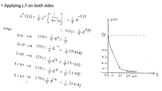
29. • The response in time domain is given by
• The eqn (1) is the response of the closed loop 1st
order system for unit step i/p.
• For step i/p of step value, A, the eqn (1) is multiplied by A.

31. Response of 1st
Order System for Unit Ramp I/p
• Consider a 1st
order system as shown in fig below.
• The T.F is given by
• The i/p applied to the system is a unit ramp i/p

32. • Taking partial fraction expansion, we have

35. Response of 1st
Order System with Unit Impulse I/p
• Consider the closed loop T.F of 1st
order system is given by
• For impulse function, we have
r(t) = δ(t)
R(s) = 1
• Substitute R(s) value in eqn (1)

36. • Applying L.T on both sides

37. Response of 1st
Order System for Parabolic I/p
• Consider the closed loop T.F of 1st
order system is given by
• Applying partial fraction expansion on above eqn, we have

41. Second Order System
• The closed loop 2nd
order system is shown in below fig.
• Where,

42. • The damping ratio is defined as the ratio of the actual damping to the critical
damping. The response c(t) of 2nd
order system depends on the value of damping
ratio.
• Depending on the value of ζ , the system can be classified into four cases.
Case 1: Undamped System, ζ = 0
Case 2: Under damped system, 0< ζ < 1
Case 3: Critically damped system, ζ = 1
Case 4: Over damped system, ζ > 1

43. • The C.E of the 2nd
order system is,
s2
+ 2ζωns + ωn
2
= 0 ------ (2)
• It is a quadratic eqn & the roots of this eqn is given by,

44. • Here ωd is called damped frequency of oscillation of the system & its unit is
rad/sec.

45. Response of Undamped 2nd
Order System for Unit Step I/p
• The standard form of closed loop T.F of 2nd
order system is,
• For undamped system, ζ = 0
• When i/p is unit step, r(t) =1 and R(s) = 1/s.
• By partial fraction expansion,

46. • A is obtained by multiplying C(s) by s and letting s = 0
• B is obtained by multiplying C(s) by (s2
+ ωn
2
) and letting s2
= ωn
2 or
s = jωn
c(t) = 1 – cosωnt

48. Note: Every practical system has some amount of damping. Hence undamped
systems does not exist in practice.
For closed loop undamped 2nd
order system,
Unit step response = (1 – cosωnt)
Step response = A(1 – cosωnt)

49. Response of critically damped 2nd
Order System for Unit Step I/p
• The standard form of closed system T.F of 2nd
order system is,
• For critically damping system, ζ = 1
• When i/p is unit step, r(t) = 1 and R(s) = 1/s. Therefore the response in s-domain,
• By partial fraction expansion, we can write

50. • By applying the Inverse L.T, we get the response in time domain, i.e,

51. • The above eqn is the response of critically damped closed loop 2nd
order system
for unit step i/p.
• For step i/p of a step value A, the above eqn should be multiplied by A.

52. Response of Under damped 2nd
Order System for Unit Step I/p
• The standard form of closed system T.F of 2nd
order system is,
• For under damped system, 0 < ζ < 1 and roots of the denominator(C.E) are
complex conjugate.
The roots of the denominator is,

53. • The response in s-domain,
• For unit step i/p, r(t) = 1 and R(s) = 1/s.
• By partial fraction expansion,
• A is obtained by multiplying C(s) by s and letting s = 0.
• To solve for B & C, cross multiply above eqn and equate like power of s.
• On cross multiplication of above eqn, after substituting A = 1, we get

56. • The above eqn is response of under damped closed loop 2nd
order system for unit
step i/p. For step i/p of value A, the above eqn should be multiplied by A.

57. Response of Over damped 2nd
Order System for Unit Step I/p
• The standard form of closed loop T.F of 2nd
order system is,
• For over damped system, ζ >1. the roots of the denominator of T.F are real and
distinct. Let the roots of the denominator be sa, sb

58. • For step i/p r(t) = 1 and R(s) = 1/s.
• By partial fraction expansion, we can write

60. • The above eqn is the response of overdamped closed loop system for unit step
i/p. For step i/p of value A, the above eqn is multiplied by A.

62. Time Domain Specifications
• The desired performance characteristics of control systems are specified in terms
of time domain specifications.
• Systems with energy storage elements cannot respond instantaneously and will
exhibit transient responses, whenever they are subjected to i/p or disturbances.
• The desired performance characteristics of a system of any order may be
specified in terms of the transient response to a unit step signal.
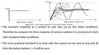
• The response of a 2nd
order system for unit step i/p with various values of
damping ratio is shown in below fig.

63. • The transient response of a system to unit step i/p on the initial conditions.
Therefore to compare the time response of various systems it is necessary to start
with standard initial conditions.
• The most practical standard is to start with the system at rest and so o/p and all
time derivatives before t = 0 will be zero.

64. • The transient response of a practical control system often exhibits damped
oscillation before reaching steady state. A typical damped oscillatory response of
a system is shown in fig.,

65. • The transient response characteristics of a control system to a unit step i/p is
specified in terms of the following time domain specifications.
1. Delay time, td
2. Rise time, tt
3. Peak time, tp
4. Maximum Peak overshoot, Mp
5. Settling time, ts
Delay time, (td): It is the time taken for response to reach 50% of the final value,

66. Rise time, (tt): It’s the time taken for response to raise from 0 to 100% for the very
1st
time. For under damped system, the rise time is calculated from 0 to 100%. But
for over damped system it’s the time taken by the response to raise from 10% to
90%. For critically damped system, it’s the time taken for response to raise from 5%
to 95%.
Peak time, (tp): It’s the time takem for the response to reach the peak value the
very 1st
time. Or It’s the time taken for the response to reach the peak overshoot,
Mp.
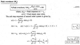
Peak overshoot, (Mp): It is identified as the ratio of maximum peak value to the

67. • Let, c() = Final value of c(t).
c(tp) = Max. Value of c(t).
Now, peak overshoot,
% Peak overshoot,
Settling time, (ts): It is defined as the time taken by the response to reach and stay
within a specified error. It is usually expressed as % of final value. The usual
tolerable error is 2% or 5% of the final value.

68. Expressions for Time Domain Specifications
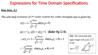
Rise time, (tr)
The unit step response of 2nd
order system for under damped case is given by,

70. Peak time, (tp)
• To find expression for peak time, tp, differentiate c(t) w.r.to t and equate to 0.
• The unit step response of under damped 2nd
order system is given by,
• Differentiate c(t) w.r.to t.

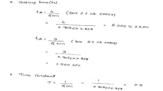
75. Settling time, (ts)
• The response of 2nd
order system has two components. They are,
1. Decaying exponential component,
2. Sinusoidal component, sin(ωdt + Ɵ).
• In this the decaying exponential term dampens or reduces the oscillations
produced by sinusoidal component. Hence the settling time is decided by the
exponential component.
• The settling time can be found out by equating exponential component to
percentage tolerance errors.

76. For 2% tolerance error band, at

77. Delay time, (td)
td =

121. Type Number of Control Systems
• The type number is specified for loop T.F G(s)H(s). The no.of poles of the loop T.F
lying at the origin decides the type number of the system.
• In general, if N is the no.of poles at the origin then the type number is N. The
loop T.F can be expressed as a ratio of two polynomials in s.

122. • The value of N in the denominator polynomial of loop T.F shown in above eqn
decides the type number of the system.
If N = 0, then the system is type – 0 system
If N = 1, then the system is type – 1 system
If N = 2, then the system is type – 2 system
If N = 3, then the system is type – 3 system
.
.

123. Steady State Error
• The steady state error is the value of error signal e(t), when t tends to infinity. The steady state
error is a measure of the system accuracy.
• These errors arise from the nature of i/ps, type of system and from non linearity of system
components.
• The steady state performance of stable control system is generally judged by its steady state
error to step, ramp and parabolic i/ps.
• Consider a closed loop system shown in fig.,
Let, R(s) = I/p signal, E(s) = Error signal,
C(s) = O/P signal or response
C(s)H(s) = feed back signal,

124. • The error signal, e(t) = R(s) – C(s)H(s)
• The O/P signal, C(s) = E(s)G(s)
• On substituting for C(s) from above eqns, we get,
E(s) = R(s) – [E(s)G(s)]H(s)
E(s) + E(s)G(S)H(s) = R(s)
E(s)[1+G(s)H(s)] = R(s)
Let, e(t) = error signal in time domain.

126. Static Error Constants
• When a control system is excited with standard i/p signal, the steady state error may be zero,
constant or infinity. The value of steady state error depends on the type number and the i/p
signal.
• Type – 0 system will have a constant steady state error when the i/p is step signal.
• Type- 1 system will have a constant steady state error when the i/p is ramp signal or velocity
signal.
• Type – 2 system will have a constant steady state error when the i/p is parabolic signal or
acceleration signal.
• For 3 cases mentioned above the SSE is associated with one of the constants defined as
follows,

127. The Kp, Kv, Ka are in general called static error constants.

128. Steady State Error when the i/p is Unit Step
Steady state error,
When the i/p is unit step, R(s) = 1/s.
The constant Kp is called positional error constant.
Type – 0 system:

129. • Hence in type – 0 systems when the i/p is unit step there will be aconstant steadt
state error.
Type – 1 system:
• In systems with type number 1 and above, for unit step i/p the value of Kp is
infinity and so the steady state error is zero.

130. Steady State Error when the i/p is Unit Ramp

132. Steady State Error when the i/p is Unit Parabolic

147. Controllers
• A controller is a device introduced in the system to modify the error signal and to produce a control signal. The
manner in which the controller produces the control signal is called control action.
• The controller modifies the transient response of the system. The controllers may be electrical, electronic,
hydraulic or pneumatic, depending on the Nature of the signal & the system. Only electronic controllers are
discussed here.
• The following six basic control actions are very common among industrial analog controllers.
They are

148. 1. Two Position or ON-OFF control action.
2. Proportional control action.
3. Integral control action.
4. Proportional – plus – Integral control action.
5. Proportional – plus – Derivative control action.
6. Proportional – plus – Integral - plus – Derivative control action.
• Depending on the control actions provided, the controllers can be classified as
follows

149. 1. Two Position or ON-OFF controllers.
1. Proportional controllers.
2. Integral controllers.
3. Proportional – plus – Integral controllers.
4. Proportional – plus – Derivative controllers.
5. Proportional – plus – Integral - plus – Derivative controllers.
ON – OFF or Two Position Controller:
• The ON – OFF or Two position controller has only two fixed positions. They are
ON or OFF.

150. • The ON-OFF control system is very simple in construction and hence less
expensive. For this reason, it is widely used in both industrial & domestic control
systems.
• The ON-OFF control action may be provided by a relay. There are different types
of relay. The most popular one is electromagnetic relay.
• It is a device which has NO(Normally Open) and NC(Normally closed) contacts,
whose opening & closing are controlled by the relay coil.
• When the relay coil is excited, the relay operates & the contacts change their
positions i.e., NO -> NC and NC -> NO.

151. • Let the o/p signal from the controller be u(t) and the actuating error signal be
e(t). In this controller, u(t) remains at either a maximum or minimum value.
u(t) = u1 ; for e(t) < 0
= u2 ; for e(t) > 0

152. Proportional Controller (P – Controller):
• The proportional controller is a device that produces a control signal, u(t)
proportional to the i/p error signal, e(t).
In P – Controller u(t) e(t)
∝
Therefore, u(t) = Kp e(t) …….(1)
where Kp = Proportional gain or constant
On taking L.Tof above eqn, we get,
U(s) = KpE(s) ……….(2)
Therefore, Kp = U(s)/E(s) ……..(3)

153. • The eqn (2) gives the o/p of the P-Controller for the i/p E(s) and eqn (3) is the T.F
of the P-controller. The block diagram of the P-controller is shown in fig.,
(Or)

156. • The offset can be reduced by increasing proportional gain, but may also cause
increase oscillations for higher order systems.
• The offset, often termed as “steady state error” can also be obtained by from the
error T.F and the error function e(t) can be expressed in terms of the L.T form:

157. Advantages:
• Steady state tracking is accurate.
• Rejects the disturbance signal.
• Relative stability
• Increase the loop gain but the system is low sensitivity.
Disadvantages:
• The P-controller leads to constant steady state error,

158. Integral Controller (I – Controller):
• The integral controller is a device that produces a control signal u(t) which is
proportional to integral of the i/p error signal, e(t).
In I-controller, u(t) ∝ -------------- (1)
Therefore, u(t) = Ki dt -------------- (2)
Where, Ki = Integral Gain or constant.
• On taking L.T of eqn (2) with zero initial conditions we get,

159. • The eqn (2) gives the o/p of the I-controller for the i/p E(s) & eqn (3) is the T.F of
the I-controller. The block diagram of I-controller is shown in fig.,
• Or

160. • From the 1st
observation, it can be seen that with I-controller, the order of the
closed loop system increases by one. This increase in order may causes instability
of closed loop system, if the process is of higher order dynamics.
• For a step i/p, r(s)=A/s.

161. • So, the major advantage of this integral control action is that the steady state
error due to step i/p reduces to zero. But simultaneously, the system response is
generally slow, oscillatory and unless properly designed, sometimes even
unstable.
• The step response of this closed loop system with integral action is shown in fig.,

162. Proportional plus Integral Controller (PI – Controller):
• This PI-controller produces an o/p signal consisting of two terms: one
proportional to error signal and the other proportional to the integral of error
signal.
In PI-controller, u(t) ∝];
Therefore, u(t) = Kp e(t) +
Where Kp = Proportional Gain,
Ti = Integral time.
On taking L.T of above eqn with zero initial conditions, we get,

163. U(s) = Kp E(s) +
U(s) = E(s) Kp [1+ ]
Therefore, = Kp [1+ ]
• It is evident from the above discussions that the PI action provides the
dual advantages of fast response due to P-action and the zero steady
state error due to I-action.
• The error T.F of the above system can be expressed as:

164. • In the same way as an integral control, we can conclude that steady state error
would be zero for PI-action. Besides, the closed loop characteristics eqn for PI
action is:

165. • Comparing these two, one can easily observe that, by varying the term Kp, the
damping constant can be increased.
• So, we can conclude that by using PI control, the steady state error can be
brought down to zero, and simultaneously, the transient response can be
improved.
• The o/p response due to (i). P, (ii). I, (iii). P-I control for the same plant can be
compared from the sketch shown in below fig.,

166. Effect of PI-controller on the performance of the system
• The PI-controller increases the order of the system by one, hence resulting in the
elimination or reduces of the steady state error produced due to the
proportional action.
• The proportional action increase the Loop gain and thus make the system less
sensitive to variations of system parameters.
• It improves the steady state tracking accuracy and rejection of disturbance signal.
But the proportional action introduces steady state error. This steady state error
is minimized or eliminated by the integral action.

167. Proportional plus Derivative Controller (PD – Controller):
• This controller produces an o/p signal consisting of two terms: one proportional
to error and the other proportional to the derivative of error signal.
In PD-controller, u(t) ∝ [ e(t) + ];
u(t) =Kp e(t) + Kp Td
Where, Kp = Proportional gain,
Td = Derivative time.
• On taking L.T of above eqn with zero initial conditions, we get,

168. U(s) = Kp E(s) +
= Kp[1 + Tds]
The block diagram of PD- controller is,
• The derivative control acts on rate of change of error and not on the actual error signal. The
derivative action is effective only during transient periods and so it does not produce corrective
measures for any constant error.
• Hence, the derivative controller is never used alone, but it is employed in association with
proportional & integral controllers.
Kp[1 + Tds]

169. • The derivative controllers does not affect the steady state error directly, but
anticipates the error, initiates an early corrective action and tends to increase the
stability of the system.
• While derivative control action has an advantage of being anticipatory it has the
disadvantage that it amplifies noise signals and may cause a saturation effect in
the actuator.
• The step response with P & PD controllers
are compared in shown fig.,

170. Effect of PD-controller on the performance of the system
• The performance of the system is affected by PD controller in the following ways.
1. The PD-controller reduces the Peak Overshoot.
2. It reduces the rise time and settling time.
3. It also increases the damping ratio.
4. There will be no affect of PD-controller on natural frequency.
5. Steady state error is not affected and type of the system remains unchanged.
6. it develops noise signal and causes saturation effect.

171. Proportional plus Integral plus Derivative Controller (PID – Controller):
• The PID controllers produce an o/p consisting of three terms: one proportional to error
signal, another one proportional to integral of error signal and the third one proportional
to the derivative of error signal.
• In PID-controller, u(t) ∝ [ e(t) + + ]
Therefore, u(t) = Kpe(t) + + Kp Td
Where, Kp = Proportional gain,
Ti = Integral time,
Td = Derivative time
• on taking L.T eith zero initial conditions, we get,

172. U(s) = Kp E(s) + Kp
= Kp[1 + Tds + ]
• The block diagram of PID-controller is shi=own in below fig.,
• The proportional integral derivative controller is used to improve the stability of
the control system and to decrease steady state error.
Kp[1 + Tds + ]