The Laplace transform allows solving differential equations using algebra by transforming differential operators into algebraic operations. It transforms a function of time (f(t)) into a function of a complex variable (F(s)), allowing differential equations describing systems to be solved for variables of interest. Key properties include linearity, time and frequency shifting, and relationships between derivatives, integrals, and the Laplace transform that enable solving differential equations by taking the transform, performing algebra, and applying the inverse transform.

1. Laplace Transform

2. Why use Laplace Transforms?
 Find solution to differential equation using algebra
 Relationship to Fourier Transform allows easy way to
characterize systems
 No need for convolution of input and differential equation
solution
 Useful with multiple processes in system

3. How to use Laplace
 Find differential equations that describe system
 Obtain Laplace transform
 Perform algebra to solve for output or variable of interest
 Apply inverse transform to find solution

4. What are Laplace transforms?









j
j
st
st
dsesF
j
sFLtf
dtetftfLsF


)(
2
1
)}({)(
)()}({)(
1
0
 ‘t’ is real, ‘s’ is complex!
 Inverse requires complex analysis to solve
 Note “transform”: f(t)  F(s), where t is integrated
and s is variable
 Conversely F(s)  f(t), t is variable and s is
integrated
 Assumes f(t) = 0 for all t < 0

5. Evaluating F(s) = L{f(t)}
 Hard Way – do the integral

 



 











0
0 0
)(
0
)sin()(
sin)(
1
)(
)(
1
)10(
1
)(
1)(
dttesF
ttf
as
dtedteesF
etf
ss
dtesF
tf
st
tasstat
at
st
let
let
let
Integrate by parts

6. Evaluating F(s)=L{f(t)}- Hard Way
remember
  vduuvudv
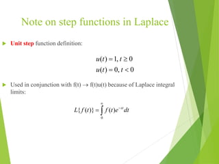
)cos(,)sin(
,
tvdttdv
dtsedueu stst

 

 


 



0
0 0
0
)cos()1(
)cos()cos([)sin( ]
dttese
dttestedtte
stst
ststst
)sin(,)cos(
,
tvdttdv
dtsedueu stst

 










00
0
0
)sin()0()sin()sin([
)cos(
] dttesedtteste
dtte
stststst
st 2
0
0
2
0 0
2
1
1
)sin(
1)sin()1(
)sin(1)sin(
s
dtte
dttes
dttesdttse
st
st
stst






 




 

let
let
Substituting, we get:
It only gets worse…

7. Evaluating F(s) = L{f(t)}
 This is the easy way ...
 Recognize a few different transforms
 See table 2.3 on page 42 in textbook
 Or see handout ....
 Learn a few different properties
 Do a little math

8. Table of selected Laplace Transforms
1
1
)()()sin()(
1
)()()cos()(
1
)()()(
1
)()()(
2
2








s
sFtuttf
s
s
sFtuttf
as
sFtuetf
s
sFtutf
at

9. More transforms
1
!
)()()( 
 n
n
s
n
sFtuttf
66
5
2
1
120!5
)()()(,5
!1
)()()(,1
1!0
)()()(,0
ss
sFtuttfn
s
sFttutfn
ss
sFtutfn



1)()()(  sFttf 

10. Note on step functions in Laplace




0
)()}({ dtetftfL st
 Unit step function definition:
 Used in conjunction with f(t)  f(t)u(t) because of Laplace integral
limits:
0,0)(
0,1)(


ttu
ttu

11. Properties of Laplace Transforms
 Linearity
 Scaling in time
 Time shift
 “frequency” or s-plane shift
 Multiplication by tn
 Integration
 Differentiation

12. Properties: Linearity
)()()}()({ 22112211 sFcsFctfctfcL 
Example :
1
1
)
1
)1()1(
(
2
1
)
1
1
1
1
(
2
1
}{
2
1
}{
2
1
}
2
1
2
1
{
)}{sinh(
22













ss
ss
ss
eLeL
eey
tL
tt
tt
Proof :
)()(
)()(
)]()([
)}()({
2211
0
22
0
11
22
0
11
2211
sFcsFc
dtetfcdtetfc
dtetfctfc
tfctfcL
stst
st













13. )(
1
)}({
a
s
F
a
atfL 
Example :
22
22
2
2
)(
1
)1
)(
1
(
1
)}{sin(












s
s
s
tL Proof :
)(
1
)(
1
1
,,
)(
)}({
0
)(
0
a
s
F
a
dueuf
a
du
a
dt
a
u
tatu
dteatf
atfL
a
u
a
s
st










let
Properties: Scaling in Time

14. Properties: Time Shift
)()}()({ 0
00 sFettuttfL st

Example :
as
e
tueL
s
ta





10
)10(
)}10({ Proof :
)()(
)(
,
)(
)()(
)}()({
00
0
0
0
0
0
)(
00
0
0
00
00
sFedueufe
dueuf
tutttu
dtettf
dtettuttf
ttuttfL
stsust
t
tus
t
st
st



















let

15. Properties: S-plane (frequency) shift
)()}({ asFtfeL at

Example :
22
)(
)}sin({






as
teL at Proof :
)(
)(
)(
)}({
0
)(
0
asF
dtetf
dtetfe
tfeL
tas
stat
at











16. Properties: Multiplication by tn
)()1()}({ sF
ds
d
tftL n
n
nn

Example :
1
!
)
1
()1(
)}({



n
n
n
n
n
s
n
sds
d
tutL Proof :
)()1()()1(
)()1(
)(
)()}({
0
0
0
0
sF
s
dtetf
s
dte
s
tf
dtettf
dtetfttftL
n
n
nst
n
n
n
st
n
n
n
stn
stnn
























17. The “D” Operator
1. Differentiation shorthand
2. Integration shorthand
)()(
)(
)(
2
2
2
tf
dt
d
tfD
dt
tdf
tDf


)()(
)()(
tftDg
dttftg
t

 
)()(
)()(
1
tfDtg
dttftg
a
t
a


 if
then then
if

18. Properties: Integrals
s
sF
tfDL
)(
)}({ 1
0 
Example :
)}{sin(
1
1
)
1
)(
1
(
)}cos({
22
1
0
tL
ss
s
s
tDL





Proof :
let
stst
st
e
s
vdtedv
dttfdutgu
dtetgtL
tfDtg









1
,
)(),(
)()}{sin(
)()(
0
1
0



 
t
stst
dttftg
s
sF
dtetf
s
etg
s
0
0
)()(
)(
)(
1
])(
1
[




0
)()( dtetft st
If t=0, g(t)=0
for so
slower than


0
)()( tgdttf 0st
e

19. Properties: Derivatives
(this is the big one)
)0()()}({ 
 fssFtDfL
Example :
)}sin({
1
1
1
)1(
1
1
)0(
1
)}cos({
2
2
22
2
2
2
2
tL
s
s
ss
s
s
f
s
s
tDL














Proof :
)()0(
)()]([
)(,)(
,
)()}({
0
0
0
ssFf
dtetfstfe
tfvdttf
dt
d
dv
sedueu
dtetf
dt
d
tDfL
stst
stst
st













let

20. Difference in
 The values are only different if f(t) is not continuous @ t=0
 Example of discontinuous function: u(t)
)0(&)0(),0( fff 
1)0()0(
1)(lim)0(
0)(lim)0(
0
0









uf
tuf
tuf
t
t

21. ?)}({ 2
tfDL
)0(')0()()0('))0()((
)0(')}({)0()()}({
)0(')0()0(),()(
2
2
fsFsFsffssFs
ftDfsLgssGtgDL
fDfgtDftg


let
)0()0()0(')0()()}({ )'1()'2()2()1( 
 nnnnnn
fsffsfssFstfDL 
NOTE: to take
you need the value @ t=0 for
called initial conditions!
We will use this to solve differential equations!

)(),(),...(),( 21
tftDftfDtfD nn
)}({ tfDL n
Properties: Nth order derivatives

22. Properties: Nth order derivatives
)0()()}({ fssFtDfL 
)}({ 2
tfDL
)0()()}({)}({)(
)0(')0(
)()(
)0()()}({
)()()()( 2
fssFtDfLtgLsG
fg
tDftg
gssGtDgL
tfDtDgandtDftg





)0(')0()()0(')]0()([)0()()}({ 2
fsfsFsffssFsgssGtDgL 
.),(),( 43
etctfDtfD
Start with
Now apply again
let
then
remember
Can repeat for
)0()0()0(')0()()}({ )'1()'2()2()1( 
 nnnnnn
fsffsfssFstfDL 