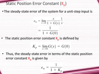
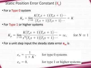
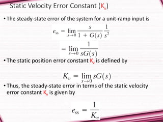
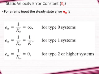
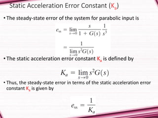
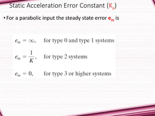
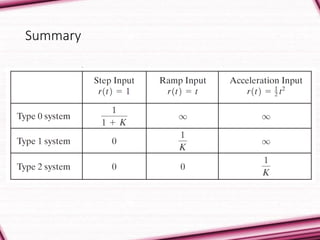
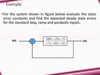
Steady State Error
Introduction
• Steady-state error is defined as the difference between the input
(command) and the output of a system in the limit as time goes to infinity
(i.e. when the response has reached steady state).
• Any physical control system inherently suffers steady-state error in
response to certain types of inputs.
• A system may have no steady-state error to a step input, but the same
system may exhibit nonzero steady-state error to a ramp input.
• Whether a given system will exhibit steady-state error for a given type of
input depends on the type of open-loop transfer function of the system.
• Control systems may be classified according to their ability to follow step
inputs, ramp inputs, parabolic inputs, and so on.
• The magnitudes of the steady-state errors due to these individual inputs
are indicative of the goodness of the system.
Classification of Control Systems
• Consider the unity-feedback control system with the following open-loop
transfer function
• It involves the term sN in the denominator,
representing N poles at the origin.
• A system is called type 0, type 1, type 2, ... , if
N=0, N=1, N=2, ... , respectively.
Classification of Control Systems
• As the type number is increased, accuracy is improved.
• However, increasing the type number aggravates the stability problem.
• A compromise between steady-state accuracy and relative stability is
always necessary.
Steady State Error of Unity Feedback Systems
• Consider the system shown in following figure.
• The closed-loop transfer function is
Steady State Error of Unity Feedback Systems
• The transfer function between the error signal E(s) and the
input signal R(s) is
)()(
)(
sGsR
sE


1
1
• The final-value theorem provides a convenient way to find
the steady-state performance of a stable system.
• Since E(s) is
• The steady state error is
Static Error Constants
• The static error constants are figures of merit of control systems. The higher
the constants, the smaller the steady-state error.
• In a given system, the output may be the position, velocity, pressure,
temperature, or the like.
• Therefore, in what follows, we shall call the output “position,” the rate of
change of the output “velocity,” and so on.
• This means that in a temperature control system “position” represents the
output temperature, “velocity” represents the rate of change of the output
temperature, and so on.
Static Position Error Constant (Kp)
• The steady-state error of the system for a unit-step input is
• The static position error constant Kp is defined by
• Thus, the steady-state error in terms of the static position
error constant Kp is given by
Static Position Error Constant (Kp)
• For a Type 0 system
• For Type 1 or higher systems
• For a unit step input the steady state error ess is
Static Velocity Error Constant (Kv)
• The steady-state error of the system for a unit-ramp input is
• The static position error constant Kv is defined by
• Thus, the steady-state error in terms of the static velocity
error constant Kv is given by
Static Velocity Error Constant (Kv)
• For a Type 0 system
• For Type 1 systems
• For type 2 or higher systems
Static Velocity Error Constant (Kv)
• For a ramp input the steady state error ess is
Static Acceleration Error Constant (Ka)
• The steady-state error of the system for parabolic input is
• The static acceleration error constant Ka is defined by
• Thus, the steady-state error in terms of the static acceleration error
constant Ka is given by
Static Acceleration Error Constant (Ka)
• For a Type 0 system
• For Type 1 systems
• For type 2 systems
• For type 3 or higher systems
Static Acceleration Error Constant (Ka)
• For a parabolic input the steady state error ess is
Summary
Example
•For the system shown in figure below evaluate the static
error constants and find the expected steady state errors
for the standard step, ramp and parabolic inputs.
C(S)R(S) -
))((
))((
128
52100
2


sss
ss
Example (Steady Sate Errors)
pK vK 410.aK
0
0
090.
Example (evaluation of Static Error Constants)
))((
))((
)(
128
52100
2



sss
ss
sG
)(lim sGK
s
p
0










 ))((
))((
lim
128
52100
2
0 sss
ss
K
s
p
pK
)(lim ssGK
s
v
0










 ))((
))((
lim
128
52100
2
0 sss
sss
K
s
v
vK
)(lim sGsK
s
a
2
0












 ))((
))((
lim
128
52100
2
2
0 sss
sss
K
s
a
410
12080
5020100
.
))((
))((








aK

6. steady state error

  • 1.
  • 2.
    Introduction • Steady-state erroris defined as the difference between the input (command) and the output of a system in the limit as time goes to infinity (i.e. when the response has reached steady state). • Any physical control system inherently suffers steady-state error in response to certain types of inputs. • A system may have no steady-state error to a step input, but the same system may exhibit nonzero steady-state error to a ramp input. • Whether a given system will exhibit steady-state error for a given type of input depends on the type of open-loop transfer function of the system. • Control systems may be classified according to their ability to follow step inputs, ramp inputs, parabolic inputs, and so on. • The magnitudes of the steady-state errors due to these individual inputs are indicative of the goodness of the system.
  • 3.
    Classification of ControlSystems • Consider the unity-feedback control system with the following open-loop transfer function • It involves the term sN in the denominator, representing N poles at the origin. • A system is called type 0, type 1, type 2, ... , if N=0, N=1, N=2, ... , respectively.
  • 4.
    Classification of ControlSystems • As the type number is increased, accuracy is improved. • However, increasing the type number aggravates the stability problem. • A compromise between steady-state accuracy and relative stability is always necessary.
  • 5.
    Steady State Errorof Unity Feedback Systems • Consider the system shown in following figure. • The closed-loop transfer function is
  • 6.
    Steady State Errorof Unity Feedback Systems • The transfer function between the error signal E(s) and the input signal R(s) is )()( )( sGsR sE   1 1 • The final-value theorem provides a convenient way to find the steady-state performance of a stable system. • Since E(s) is • The steady state error is
  • 7.
    Static Error Constants •The static error constants are figures of merit of control systems. The higher the constants, the smaller the steady-state error. • In a given system, the output may be the position, velocity, pressure, temperature, or the like. • Therefore, in what follows, we shall call the output “position,” the rate of change of the output “velocity,” and so on. • This means that in a temperature control system “position” represents the output temperature, “velocity” represents the rate of change of the output temperature, and so on.
  • 8.
    Static Position ErrorConstant (Kp) • The steady-state error of the system for a unit-step input is • The static position error constant Kp is defined by • Thus, the steady-state error in terms of the static position error constant Kp is given by
  • 9.
    Static Position ErrorConstant (Kp) • For a Type 0 system • For Type 1 or higher systems • For a unit step input the steady state error ess is
  • 10.
    Static Velocity ErrorConstant (Kv) • The steady-state error of the system for a unit-ramp input is • The static position error constant Kv is defined by • Thus, the steady-state error in terms of the static velocity error constant Kv is given by
  • 11.
    Static Velocity ErrorConstant (Kv) • For a Type 0 system • For Type 1 systems • For type 2 or higher systems
  • 12.
    Static Velocity ErrorConstant (Kv) • For a ramp input the steady state error ess is
  • 13.
    Static Acceleration ErrorConstant (Ka) • The steady-state error of the system for parabolic input is • The static acceleration error constant Ka is defined by • Thus, the steady-state error in terms of the static acceleration error constant Ka is given by
  • 14.
    Static Acceleration ErrorConstant (Ka) • For a Type 0 system • For Type 1 systems • For type 2 systems • For type 3 or higher systems
  • 15.
    Static Acceleration ErrorConstant (Ka) • For a parabolic input the steady state error ess is
  • 16.
  • 17.
    Example •For the systemshown in figure below evaluate the static error constants and find the expected steady state errors for the standard step, ramp and parabolic inputs. C(S)R(S) - ))(( ))(( 128 52100 2   sss ss
  • 18.
    Example (Steady SateErrors) pK vK 410.aK 0 0 090.
  • 19.
    Example (evaluation ofStatic Error Constants) ))(( ))(( )( 128 52100 2    sss ss sG )(lim sGK s p 0            ))(( ))(( lim 128 52100 2 0 sss ss K s p pK )(lim ssGK s v 0            ))(( ))(( lim 128 52100 2 0 sss sss K s v vK )(lim sGsK s a 2 0              ))(( ))(( lim 128 52100 2 2 0 sss sss K s a 410 12080 5020100 . ))(( ))((         aK