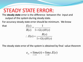
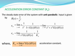
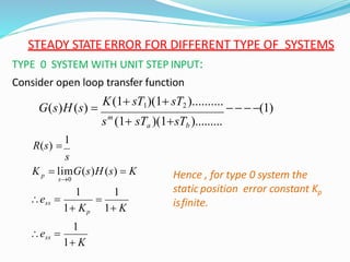
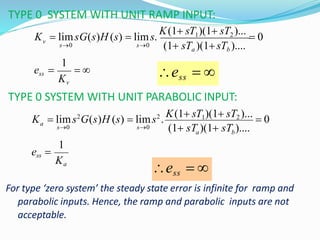
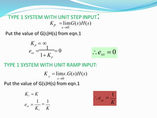
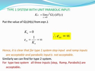
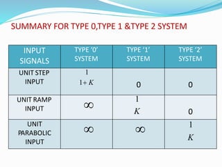
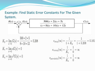
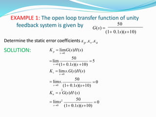
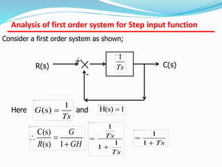
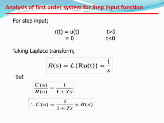
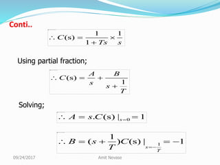
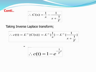
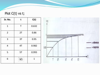
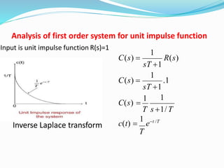
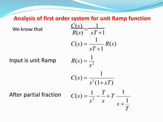
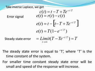
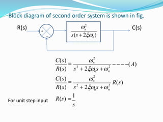
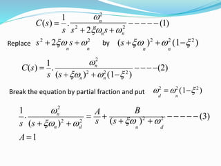
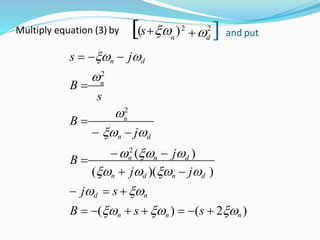
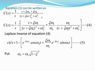
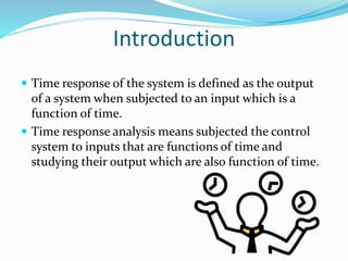
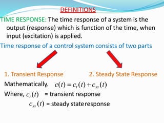
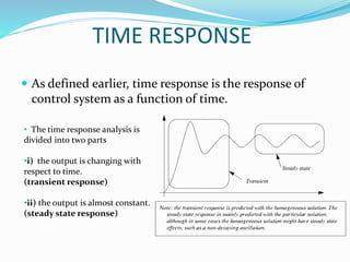
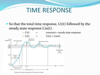
This document provides an analysis of the time response of control systems. It defines time response as the output of a system over time in response to an input that varies over time. The time response analysis is divided into transient response, which decays over time, and steady state response. Different types of input signals are described, including step, ramp, and sinusoidal inputs. Methods for analyzing the first and second order systems are presented, including determining the transient and steady state response. Static error coefficients like position, velocity and acceleration constants are defined for different system types and inputs. Examples are provided to illustrate the analysis of first and second order systems.

1. TOPIC :TIME RESPONSE ANALYSIS
GROUP NAME :
1.JAIMIN ATODARIA (150990109001)
2.RAVIRAJ SOLANKI (150990109011)
GUIDED BY : MS. RICHA DUBEY

2. CONTENT
 Introduction
 Time Response
 Input Supplied System
 Steady State Response and Error
 Types Of The Systems
 Analysis Of First Order System
 Analysis Of Second Order System
 Transient Response specification
 Limitations
 Sums

3. Introduction
 Time response of the system is defined as the output
of a system when subjected to an input which is a
function of time.
 Time response analysis means subjected the control
system to inputs that are functions of time and
studying their output which are also function of time.

4. DEFINITIONS
TIME RESPONSE: The time response of a system is the
output (response) which is function of the time, when
input (excitation) is applied.
Time response of a control system consists of two parts
1. Transient Response 2. Steady State Response
Mathematically, c(t)  ct (t)  css (t)
Where, ct (t) = transient response
css (t) = steady stateresponse

5. TRANSIENT RESPONSE: The transient response is the
part of response which goes to zero as time
increases. Mathematically
Lim ct (t)  0
t
The transient response may be exponential or
oscillatory in nature.
STEADY STATE: The steady state response is the part of
the total response after transient has died.
STEADY STATE ERROR: If the steady state response of
the output does not match with the input then the
system has steady state error, denoted by ess .

6. TIME RESPONSE
 A control system generates an output or response for
given input.
 The input represents the desired response while the
output is actual response of system.
 Ex. Elevator

7.  As defined earlier, time response is the response of
control system as a function of time.
TIME RESPONSE
• The time response analysis is
divided into two parts
•i) the output is changing with
respect to time.
(transient response)
•ii) the output is almost constant.
(steady state response)

8.  So that the total time response, Ct(t) followed by the
steady state response Css(t).
 C(t) = transient + steady state response
 C(t) = Ct(t) + Css(t)
TIME RESPONSE

9.  For time response analysis of control systems, we need
to subject the system to various test inputs.
 Test input signals are used for testing how well a
system responds to known input.
 Some of standards test signals that are used are:
 Impulse
 Step
 Ramp
 Parabola
 Sinusoidal
INPUT SUPPLIED TO SYSTEM

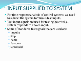
10. INPUT SUPPLIED TO SYSTEM
IMPULSE INPUT
•It is sudden change input. An impulse is
infinite at t=0 and everywhere else.
• r(t)= δ(t)= 1 t =0
= 0 t ≠o
In laplase domain we have,
• L[r(t)]= 1
STEP INPUT
•It represents a constant command such
as position. Like elevator is a step input.
•r(t)= u(t)= A t ≥0
= 0 otherwise
L[r(t)]= A/s
RAMP INPUT
• this represents a linearly increasing
input command.
•r(t) = At t ≥0,Aslope
= 0 t <0
L[r(t)]= A/s²
A= 1 then unit ramp

11. INPUT SUPPLIED TO SYSTEM
PARABOLIC INPUT
•Rate of change of velocity is
acceleration. Acceleration is a parabolic
function.
• r(t) = At ²/2 t ≥0
= 0 t <0
L[r(t)]= A/s³
SINUSOIDAL INPUT
•It input of varying and study the system
frequently response.
• r(t) = A sin(wt) t ≥0

12. STEADY STATE ERROR:
The steady state error is the difference between the input and
output of the system during steady state.
For accuracy steady state error should be minimum. We know
that
The steady state error of the system is obtained by final value theorem
1
R(s)
1 G(s)H (s)
E(s) 
R(s) 1 G(s)H (s)
E(s)

ss
t s0
e  lime(t)  lims.E(s)

13. R(s)
ss
ss
1 G(s)
e  lims.
H(s) 1
1 G(s)H (s)
e  lims.
s0
s0
For unity feedback
Thus, the steady state error depends on the input and
open loop transfer function.
R(s)

14. STATIC ERROR COEFFICIENTS
POSITIONAL ERROR CONSTANT Kp: For unit step
11
1
p
ss
ss
s0
s0
K  limG(s)H(s)
s0
1 Kp

1 limG(s)H(s)
e 
s 1 G(s)H(s)
e  lims.
1
.
Where is the positional error constantKp
input R(s)=1/s
Steady state error

15. VELOCITY ERROR CONSTANT (Kv):
Steady state error with a unit ramp input is given by R(s)=1/s2
1
ss
1 G(s)H (s)
e  Lims.R(s).
s0
v
ess
ess
1 1
11 1
2
 lim
.  lim
s 1 G(s)H (s)
 lims.
s0 sG(s)H (s) K
s0 s  sG(s)H (s)s0
Where
s0
Kv  limsG(s)H (s) velocity error coefficient

16. ACCELERATION ERROR CONSTANT (Ka):
The steady state error of the system with unit parabolic input is given
by
where,
a
ess
ess
1 1
11
s3
 lim
 lim
1 G(s)H (s)
R(s) 
1
s0 s2
G(s)H(s) K
s0 s2
 s2
G(s)H (s)
 lim s.
1
.
s0 s3
a
s0
K  lims2
G(s)H (s) acceleration constant.

17. STEADY STATE ERROR FOR DIFFERENT TYPE OF SYSTEMS
m
s (1 sTa )(1sTb ).........
TYPE 0 SYSTEM WITH UNIT STEP INPUT:
Consider open loop transfer function
G(s)H(s) 
K(1 sT1)(1 sT2 )..........
   (1)
p
ess 
ess 
1 K
1 Kp 1 K
1
1 1
K  limG(s)H (s)  K
R(s) 
1
s
s0 Hence , for type 0 system the
static position error constant Kp
isfinite.

18. TYPE 0 SYSTEM WITH UNIT RAMP INPUT:
TYPE 0 SYSTEM WITH UNIT PARABOLIC INPUT:
For type ‘zero system’ the steady state error is infinite for ramp and
parabolic inputs. Hence, the ramp and parabolic inputs are not
acceptable.
  
v
Kv
ess
1
(1 sTa )(1sTb )....
K  limsG(s)H (s)  lims.
K(1 sT1)(1 sT2 )...
 0
s0 s0
ess  
a b
a
Ka
1
ess 
(1 sT )(1 sT )....
K  lims2
G(s)H (s)  lims2
.
K(1 sT1)(1 sT2 )...
 0
s0 s0
ess  

19. TYPE 1 SYSTEM WITH UNIT STEP INPUT:
TYPE 1 SYSTEM WITH UNIT RAMP INPUT:
Put the value of G(s)H(s) from eqn.1
p
s0
K  limG(s)H(s)
ss
1 Kp
e 
1
 0
Put the value of G(s)H(s) from eqn.1
Kp  
ess  0
v
s0
K  lims.G(s)H(s)
Kv K
ess
1

1

Kv  K
ss

1
K
e

20. TYPE 1 SYSTEM WITH UNIT PARABOLIC INPUT:
Put the value of G(s)H(s) from eqn.1
Hence, it is clear that for type 1 system step input and ramp inputs
are acceptable and parabolic inputis not acceptable.
Similarly we can find for type 2 system.
For type two system all three inputs (step, Ramp, Parabolic) are
acceptable.
a
s0
K  lims2
G(s)H (s)
Ka
ess   
1
Ka  0
ess  

21. SUMMARY FOR TYPE 0,TYPE 1 &TYPE 2 SYSTEM
INPUT
SIGNALS
TYPE ‘0’
SYSTEM
TYPE ‘1’
SYSTEM
TYPE ‘2’
SYSTEM
UNIT STEP
INPUT
1
1 K 0 0
UNIT RAMP
INPUT 
1
K 0
UNIT
PARABOLIC
INPUT
  1
K

23. Example: Find Static Error Constants For The Given
System.

24. EXAMPLE 1: The open loop transfer function of unity
feedback system is given by
SOLUTION:
50
(1 0.1s)(s10)
G(s) 
Determine the static error coefficients Kp ,Kv ,Ka
50
50
50
 0
 0
5 lim
(1 0.1s)(s10)
(1 0.1s)(s10)
K  lims.G(s)H(s)
K  limG(s)H(s)
 lims2
s0
2
Ka  s G(s)H (s)
 lims.
s0
s0
v
s0 (1 0.1s)(s 10)
s0
p

26. Analysis of first order system for Step input function
Consider a first order system as shown;
+
-
R(s) C(s)
Here and
1
Ts
1
(s)G
Ts
 H(s) 1
C(s)
(s) 1
G
R GH
 

1
1
1
Ts
Ts


1
1 Ts



27. r(t) = u(t) t>0
= 0 t<0
For step input;
Taking Laplace transform;
but
Analysis of first order system for Step input function
1
(s) {Ru(t)}R L
s
 
(s) 1
(s) 1
C
R Ts


1
(s) (s)
1
C R
Ts
  


28. Using partial fraction;
Solving;
09/24/2017 Amit Nevase
Conti..
1 1
(s)
1
C
Ts s
  

(s)
1
A B
C
s
s
T
  

0. (s) | 1sA s C   
1
1
( ) (s) | 1
s
T
B s C
T 
    

29. Taking Inverse Laplace transform;
Conti..
1 1
(s)
1
C
s
s
T
  

1 1 11 1
(t) { (s)} { } { }
1
c L C L L
s
s
T
  
   

1
(t) 1
t
T
c e

  

30. Plot C(t) vs t;
Sr. No. t C(t)
1 T 0.632
2 2T 0.86
3 3T 0.95
4 4T 0.982
5 5T 0.993
6 1

31. Analysis of first order system for unit impulse function
Input is unit impulse function R(s)=1
1
1
c(t) 
1
et /T
T
T s 1/T
C(s) 
1
sT 1
C(s)  .1
sT 1
1
C(s)  R(s)
Inverse Laplace transform

32. Analysis of first order system for unit Ramp function
T
s s
1
1
R(s)
1
2
s2
s 
1
C(s) 
1

T
T
s2
(1 sT)
C(s) 
R(s) 
1
sT 1
C(s) 
R(s) sT 1
C(s)

1
Input is unit Ramp
After partial fraction
We know that

33. The steady state error is equal to ‘T’, where ‘T’ is the
time constant of the system.
For smaller time constant steady state error will be
small and speed of the response will increase.
t
e(t)  r(t)  c(t)
e(t)  t tT Tet /T

e(t)  T(1 et /T
)
 Limit(T Tet /T
)  T
Take inverse Laplace, we get
c(t)  t T Tet /T
Error signal
Steady state error

35. Block diagram of second order system is shown in fig.
R(s) C(s)
_
+
2
n
s(s  2n)
n
n
R(s)
R(s) s
R(s) s
2
n
2
2
n
2
n
2
2
n
R(s) 
1
s
C(s)

   (A)
C(s)

 2 s 

 2 s 

For unit step input

36. 2
1
2
nn
n
2
    (1)
s s  2 s 
C(s)  .
Replace s2
 2 s 2
by
n n
(s  )2
2
(12
)
n n
Break the equation by partial fraction and put 2
 2
(12
)
d n
1
.      (3)
A 1
B

A

n d
2
n
s (s  )2
2
n d
s (s  )2
2

2
(2)

n n
n
s (s  )2
2
(12
)
C(s) 
1
.

37. 22
dn (s )Multiply equation (3) by  and put
2
2
(  j )
B  n n d
(n  jd )(n  jd )
 jd  s n
B  (n  s n )  (s  2n )
B  n
 n  jd
B  n
s
s  n  jd
2

38. Equation (1) can be written as
222 

(4)
 d nd
2
dns
C(s) 
1


C(s) 
1

 (s  )(s  )
n d
s n

n
.
d
s (s  )2
2
s n n
Laplace Inverse of equation (4)
(5)




c(t) 1 e d 

d
nn
e .sin tn
d

.cos t   t t
2
d  n 1Put

39. e
dd

.cos t2
 sin t1
12
c(t) 1

.sindt
 12

cosdt c(t) 1 e
nt
nt
2
12
1
tan 
12
 sin
cos  
sin( t )

e
c(t) 1 d
nt
Put

40.     (6)

1 2 
sin(
12
12
)t  tan1e
c(t) 1 n
nt
Put the values ofd & 
    (7)

1  2 
sin(
1  2

1  2
)t  tan1e
e(t)  n
nt
Error signal for the system
e(t)  r(t)  c(t)

41. The poles are;
(i) Real and Unequal if
i.e. They lie on real axis and distinct
(ii) Real and equal if
i.e. They are repeated on real axis
(iii) Complex if
i.e. Poles are in second and third quadrant
Analysis of second order system for Step input
2
1 0  
1 
2
1 0  
1 
2
1 0  
1 

42. Relation between and pole locations
(i) Under damped
Pole Location Step Response c(t)

0 1 

43. (ii) Critically damped
Pole Location Step Response c(t)
Relation between and pole locations
1 


44. (iii) over damped
Pole Location Step Response c(t)
Relation between and pole locations
1 


45. (iv)
Pole Location
Relation between and pole locations
0 


46. TRANSIENT RESPONSE SPECIFICATIONS
 Specifications for a control system design often involve
certain requirements associated with the time
response of the closed-loop system.
 The requirements are specified by the behavior of the
controlled variable or by the control error on well
defined test signals.
 The most important test signal is a unit step on the
input of the control system and requirements are
placed on the behavior of the controlled variable

47.  The maximum overshoot is the magnitude of the overshoot after
the first crossing of the steady-state value (100%).
 The peak time is the time required to reach the maximum
overshoot.
 The settling time is the time for the controlled variable first to
reach and thereafter remain within a prescribed percentage of
the steady-state value. Common values of are 2%, 3% or 5%.
 The rise time is the time required to reach first the steady-state
value (100%).
TIME RESPONSE SPECIFICATIONS

48. Time Response Specifications

49. 1. DELAY TIME (td):
It is time required for the response to reach
50% of the final value in the first attempt.
1 0.7
d
n
t





50. 2. RISE TIME (tr): It is time required for the response to
rise from 10% to 90% of its final value for over-
damped systems and 0 to 100% for under-damped
systems.

2
2
1 
1  2
  tan1
sin 1  t  e
We know that:
c(t) 1 n
nt
Where,

51. Let response reaches 100% of desired value. Put c(t)=1
  
2
2
11 sin
1 12
 1
12
sin t  0
e
t 
e
n
n
nt
nt
 0Since, ent
sin((n
sin((n 12
)t )  sin(n)
12
)t )  0
Or,
Put n=1

52. 2
 12
 
n
tr 
(n 1  )tr    
 12
12
  tan1
 
n
rt
Or,
Or,

53. 3. PEAK TIME (tp): The peak time is the time required
for the response to reach the first peak of the time
response or first peak overshoot.
n
nt
sin 12
t  e
12
c(t) 1Since
For maximum
 0  (1)

n
nn
dt
dc(t)
 0
ent
nt
12
n
12
t 
dc(t) e
dt
sin
1 2
cos 12
t 
12

54. Since,
Equation can be written as
Equation (2) becomes
 0ent
cos
12
 sin
12
t 12
t 12
 sinnn
Put and   cos
12
t cos12
t sin  sin
n
cosn
cos
sin
cos((
sin((
12
)t )
12
)t )
n
n


55. tan((n 1 )t )  n
2
(n 1 )tp  n
2
The time to various
peak
Where n=1,2,3,…….
Peak time to first overshoot, put n=1

 12
n
pt
First minimum (undershoot) occurs at n=2
min
2
 12
n
t

56. 4. MAXIMUM OVERSHOOT (MP):
Maximum overshoot occur at peak time, t=tp
in above equation
n
nt
sin 12
t  e
12
c(t) 1

 12
n
pt

Put,





 12

12
.

sin
12
n
n
n 12
n
e
c(t) 1

57. sin



12
12
12
sin( )
12
12

12

12

c(t)  1
e
e
c(t) 1
e
c(t) 1
Put, sin  12
sin( )  sin

58. 


12

12

12

1
M  e
M 1 e
c(t) 1 e
p
p
M p  c(t)1
*100

12

M % ep

60. 5. SETTLING TIME(ts):
The settling time is defined as the time required
for the transient response to reach and stay
within the prescribed percentage error.
t  4T 
4
s

61. 6. STEADY STATE ERROR (ess): It is difference between
actual output and desired output as time ‘t’ tends to
infinity.
ss
e  Limitr(t)c(t)
t

62. LIMITATIONAS OF TIME DOMAIN
ANALYSIS
 Control system analysis is carried out in either time
domain or frequency domain. The domain of analysis
depends largely on the design requirements.
 he analysis in the frequency domain is very simple and
quick. Stability determination using a frequency
response plot can be done in very quick time with no
effort.
 In time domain analysis, the analysis becomes
cumbersome for systems of high order. In
frequency domain analysis, the order has a little effect
on the time or effort of analysis.

63. EXAMPLE 1: The open loop transfer function of a servo
system with unity feedback is given by
Determine the damping ratio, undamped natural frequency
of oscillation. What is the percentage overshoot of the
response to a unit step input.
SOLUTION: Given that
Characteristic equation
10
(s  2)(s  5)
G(s) 
10
H(s) 1
(s  2)(s 5)
G(s) 
1 G(s)H (s)  0

64. 10
 01
s2
 7s  20  0
(s  2)(s  5)
Compare with s2
 2 s 2
 0
n n
We get
*1001.92%1(0.7826)2

*0.7826
12

2* *4.472 7
  0.7826
 2
20
 e
20  4.472rad /sec
M p e
n 
n
2n  7 n 4.472rad /sec
  0.7826
M p 1.92%

65. EXAMPLE 2: A feedback system is described by the
following transfer function
H (s) Ks
The damping factor of the system is 0.8. determine the
overshoot of the system and value of ‘K’.
SOLUTION: We know that
12
G(s) 
s2
 4s 16
s2
 (4 16K)s 16  0
s2
 (4 16K)s 16R(s)
C(s)

1 G(s)H (s)
16
G(s)
R(s)
C(s)

is the characteristic eqn.

66. nn
2
n
2
Compare with
2
16
s  2 s   0
n  4rad /sec.
2n  416K
2*0.8*4  416K  K  0.15
*1001(0.8)2

M p 1.5%
*100 eM p  e
0.8
12
