Downloaded 67 times


![EXAMPLE:
+ i(t)
Lv(t)
R
L
di
dt
Ri v t
v t Ri t
( )
( ) ( ) ( )
(state equation)
Output equation
tLRtLR
L
R
L
R
eie
R
ti
s
i
ssR
sI
sVissIL
)/()/(
)0()1(
1
)(
)0(111
)(
)()]0()([
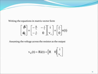
Assuming that v(t) is a unit step and knowing i(0), taking the LT of the state
equation
14](https://image.slidesharecdn.com/ssa-200222152006/85/STate-Space-Analysis-14-320.jpg)

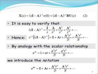
![Transfer function From State space :
DuCxy
BuAxx
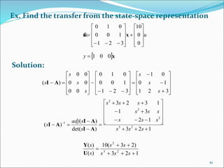
Given the state and output equations
Take the Laplace transform assuming zero initial conditions:
(1)
(2)
Solving for in Eq. (1),
or
(3)
Substitutin Eq. (3) into Eq. (2) yields
The transfer function is
)()()(
)()()(
sss
ssss
DUCXY
BUAXX
)(sX
)()()( sss BUXAI
)()()( 1
sss BUAIX
)()()()( 1
ssss DUBUAICY
)(])([ 1
ss UDBAIC
DBAIC
U
Y
1
)(
)(
)(
s
s
s
18](https://image.slidesharecdn.com/ssa-200222152006/85/STate-Space-Analysis-18-320.jpg)


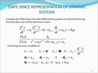
![
x
x
x
x
x
x
0 1 0 0 0 0
0 0 1 0 0 0
0 0 0 1 0 0 0
0 0 0 0 0 1 0
0 0 0 0 0 0 1
a a a a a
x
x
x
x
x
x
1
2
3
n 2
n 1
n n n 1 n 2 2 1
1
2
3
n 2
n 1
n
0
0
0
0
0
b
u
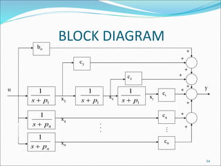
y = [1 0 0 0 0]x
0
32](https://image.slidesharecdn.com/ssa-200222152006/85/STate-Space-Analysis-32-320.jpg)


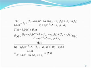


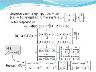
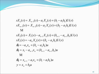
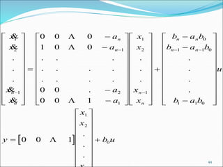
![OBSERVABLE CANONICAL FORM
s Y s b U s s a Y s bU s
s a Y s b U s a Y s b U s
Y s b U s bU s a Y s
b U s a Y s b U s a Y s
X s
n n
n n n n
s
s n n s n n
n s
n n
[ ( ) ( )] [ ( ) ( )]
[ ( ) ( )] ( ) ( )
( ) ( ) [ ( ) ( )]
[ ( ) ( )] [ ( ) ( )]
( ) [
0
1
1 1
1 1
0
1
1 1
1
1 1
1
1
0
1
bU s a Y s X s
X s b U s a Y s X s
X s b U s a Y s X s
X s b U s a Y s
Y s b U s X s
n
n s n
s n n
s n n
n
1 1 1
1
1
2 2 2
2
1
1 1 1
1
1
0
( ) ( ) ( )]
( ) [ ( ) ( ) ( )]
( ) [ ( ) ( ) ( )]
( ) [ ( ) ( )]
( ) ( ) ( )
42](https://image.slidesharecdn.com/ssa-200222152006/85/STate-Space-Analysis-42-320.jpg)


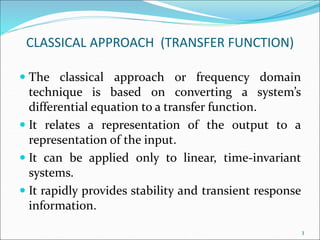
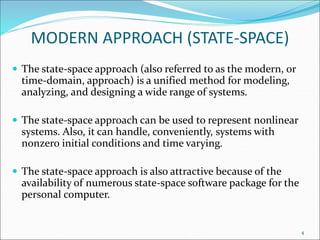
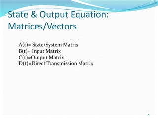
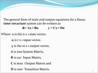
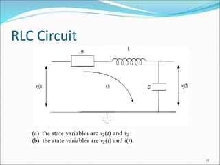
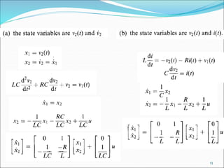
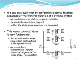
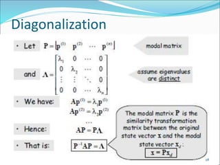
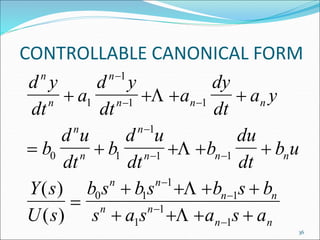
This document discusses and compares the classical/transfer function approach and the state space/modern control approach for modeling dynamical systems. The classical approach uses Laplace transforms and transfer functions in the frequency domain, while the state space approach uses matrices to represent systems of differential equations directly in the time domain. The state space approach can model nonlinear, time-varying, and multi-input multi-output systems and considers initial conditions, while the classical approach is limited to linear time-invariant single-input single-output systems. The document provides examples of modeling circuits using the state space representation.