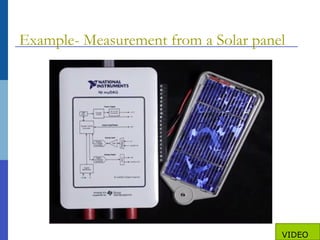
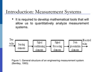
The document covers the analysis of measurement systems through time domain and frequency domain techniques. Time domain analysis focuses on the signal characteristics over time, while frequency domain analysis provides an alternative method that simplifies certain equations. An example related to voltage measurement from a solar panel is included to illustrate these concepts.

1. Time Domain and
Frequency Domain Analysis
In Measurement System
Kamble Sagar Bhikaji
Ist Sem, M.Tech (MC)
13MC12F,
NITK Surathkal.

2. Contents
1. Introduction
2. Time Domain Analysis
3. Frequency Domain Analysis
4. Example- Voltage measurement from a Solar
panel
5. Summary
6. References

3. Introduction: Measurement Systems
 It is required to develop mathematical tools that will
allow us to quantitatively analyze measurement
systems.
Figure 1. General structure of an engineering measurement system
(Bentley, 1993)

4. Introduction
Two types of mathematical tools:
1) Time Domain Analysis
- Time domain analysis examines the amplitude vs.
time characteristics of a measuring signal.
2) Frequency Domain Analysis
- Frequency domain analysis replaces the measured
signal with a group of sinusoids which, when added
together, produce a waveform equivalent to the
original.
- The relative amplitudes, frequencies, and phases
of the sinusoids are examined.

5. Time Domain Analysis
 In time-domain analysis the response of a
dynamic system to an input is expressed as a
function of time c(t).
 It is possible to compute the time response of
a system if the nature of input and the
mathematical model of the system are
known.
 The time response of a system can be
obtained by solving the differential eq.
governing the system.
 Alternatively, the response c(t) can be
obtained from the transfer function of the
system and the input to the system

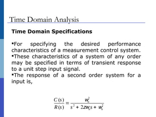
6. Time Domain Analysis
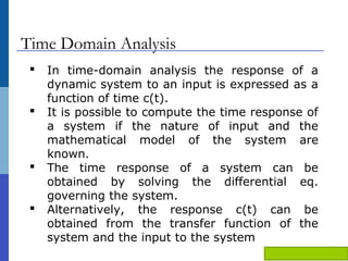
 For a closed loop transfer function,
C(s)/R(s)= G(s)/[1+G(s)H(s)]
 Response in s-domain,
C(s) = R(s)*M(s)
 Response in t-domain,
c(t) = InvLap[C(s)]

7. Time Domain Analysis
Time Domain Specifications
For specifying the desired performance
characteristics of a measurement control system.
These characteristics of a system of any order
may be specified in terms of transient response
to a unit step input signal.
The response of a second order system for a
input is,
2
2 2
( )
( ) 2
n
n n
C s
R s s s
w
zw w
=
+ +

8. Time Domain Analysis
Time Domain Specifications
1 Delay time 2 Rise time
3 Peak time 4 Peak overshoot
5 Settling time 6 Steady-state error

9. Time Domain Analysis
Time Domain Specifications
1. Delay time : It is the time required for the response to
reach 50% of the final value in first attempt.
2. Rise time : It is the time required to rise from 0 to
100% of the final value for the under damped system.
3. Peak time : It is the time required for the response to
reach the peak of time response or the peak overshoot.
4. Settling time : It is the time required for the response
to reach and stay within a specified tolerance band ( 2%
or 5%) of its final value.
5.Peak overshoot : It is the normalized difference between
the time response peak and the steady output and is
defined as,
6. Steady-state error: It indicates the error between the
actual output and desired output as ‘t’ tends to infinity.

10. Frequency Domain Analysis
 Introduction
 Advantages
- Stability of closed loop system can be
estimated
- Transfer function of complicated systems can
be determined experimentally by frequency
tests
- Effects of noise disturbance and parameter
variations are relatively easy to visualize.
- Analysis can be extended to certain nonlinear
control systems.
VIDEO

11. Frequency Domain Analysis
Frequency Domain Specifications
1 Resonant Peak
2 Resonant Frequency
3 Bandwidth
4 Cut-off rate
5 Gain Margin
6 Phase Margin

12. Frequency Domain Analysis
Frequency Domain Specifications
1 Resonant Peak- Maximum value of the closed
loop transfer function.
2 Resonant Frequency- Frequency at which
resonant peak occurs.
3 Bandwidth- range of frequencies for which the
system normalized gain is more than -3db.
4 Cut-off rate- It is the slop of the log-magnitude
curve near the cut off frequency.
5 Gain Margin- The value of gain to be added to
system in order to bring the system to the verge
of instability.
6 Phase Margin- Additional phase lag to be added
at the gain cross over freq. in order to bring the
system to the verge of instability.

13. Frequency Domain Analysis
Frequency Response Plots
Frequency domain analysis of a system can be
carried either analytically or graphically.
The various graphical techniques are
1 Bode Plot
2 Polar Plot
3 Nichols Plot
4 M and N circles
Frequency response plots are used to determine
the frequency domain specifications, to study the
stability of the system.

14. Example- Measurement from a Solar panel
VIDEO

15. Summary
Every measurement system require analysis of
its features or performance to work as a system.
Time domain analysis gives the behaviour of the
signal over time. This allows predictions and
regression models for the signal.
Frequency Analysis is much easier. Some
equations can't be solved in time domain while
they can be solved easily in frequency domain.

16. References
Control Systems- By A. Nagoor Kani, 2nd
Edition, Chapter 3 and 4.
https://6002x.mitx.mit.edu/wiki/view/TimeDom
ainVersusFrequencyDomainAnalysis
Frequency Domain in Measurements – NIglobal
channel : YouTube.
Control Systems Lectures - Time and Frequency
Domain : YouTube.

17. Any Questions ?

18. Thank You..
-Sagar Kamble
sagarkamble816@gmail.com