Downloaded 81 times


![Simplified Positive Edge triggered
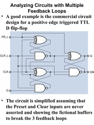
D flip-flop for analysis
(Y2·D)+(Y1·C)
Y1*
{[(Y2·D)+(Y1·C)+C‘]·Y3}+(Y1·C)
Y1
(Y1·C)'
Y3*
(Y2·D)+(Y1·C)+C' Y3
Y2*
Y2 {[(Y2·D)+(Y1·C)+C‘]·Y3}'
(Y2·D)'
Y1* = (Y2·D)+(Y1·C)
Y2* = (Y2·D)+(Y1·C)+C' = (Y2·D)+(Y1)+C'
Y3* = {[(Y2·D)+(Y1·C)+C']·Y3}+(Y1·C)
= {[(Y2·D)+(Y1)+C']·Y3}+(Y1·C)
= (Y2·Y3·D)+(Y1·Y3)+(C‘·Y3)+(Y1·C)](https://image.slidesharecdn.com/lec9-130220032608-phpapp01/85/Feedback-Sequential-Circuits-15-320.jpg)
![Simplified Positive Edge triggered
D flip-flop for analysis
(Y2·D)+(Y1·C)
Y1*
{[(Y2·D)+(Y1·C)+C‘]·Y3}+(Y1·C)
Y1
(Y1·C)'
Y3*
(Y2·D)+(Y1·C)+C' Y3
Y2*
Y2 {[(Y2·D)+(Y1·C)+C‘]·Y3}'
Y2·D'
Q = Y3* = (Y2·Y3·D)+(Y1·Y3)+(C‘·Y3)+(Y1·C)
QN = {[(Y2·D)+(Y1·C)+C']·Y3}'
= [(Y2·D)+(Y1)+C']'+Y3'
= [(Y2·D)'· (Y1)'·C'']+Y3'
= [(Y2'+D')·(Y1)'·C]+Y3'
= (Y2'·Y1'·C) + (D'·Y1'·C)+Y3'](https://image.slidesharecdn.com/lec9-130220032608-phpapp01/85/Feedback-Sequential-Circuits-16-320.jpg)


The circuit remains in state S0/10. Edge-triggered behavior means the circuit only responds to transitions of the clock signal, not its level. Since the clock did not transition from 0 to 1, the circuit ignores the changes to D and remains in the same state.