Downloaded 90 times

![Least-Squares Method Example
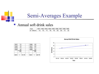
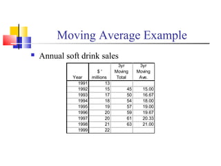
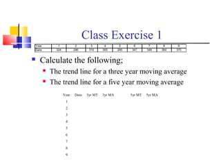
Annual soft drink sales
Find the expected sales for 2001
Year Y [x] x2
xy
1991 13 -4 16 -52
1992 15 -3 9 -45
1993 17 -2 4 -34
1994 18 -1 1 -18
1995 19 0 0 0
1996 20 1 1 20
1997 20 2 4 40
1998 21 3 9 63
1999 22 4 16 88
165 60 62
Y is the given data
X is the year value in relation to the middle year
03.1
60
62
2
=
=
=
∑
∑
b
b
x
xy
b
3.18
9
165
=
=
=
∑
a
a
n
y
a
Yt = 18.3 + 1.03x
2001 Yt = 18.3 + 1.03(6)
= 18.3 + 6.18
= 22.48
Expected sales for 2001 = $22,480,000](https://image.slidesharecdn.com/1634-timeseriesandtrendanalysis-161031145736/85/1634-time-series-and-trend-analysis-13-320.jpg)
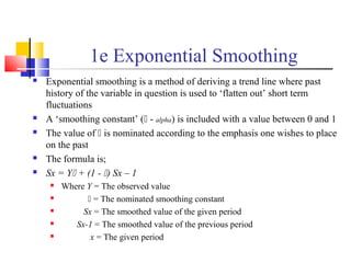
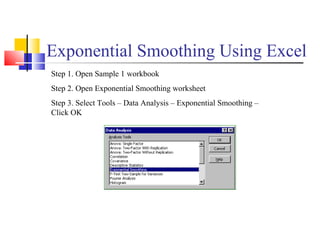
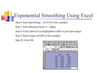
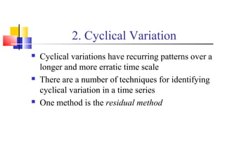

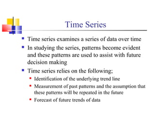
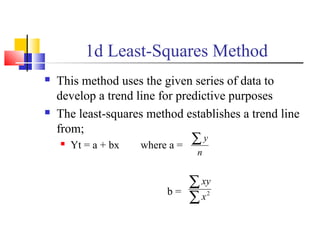
Time series analysis examines patterns in data over time. It relies on identifying trends, measuring past patterns to forecast the future, and decomposing time series into four main components: secular trends, cyclical movements, seasonal variations, and irregular variations. Secular trends represent long-term direction, while cyclical and seasonal variations have recurring patterns over different time scales. Various techniques can depict trends and identify variations, including freehand drawing, semi-averages, moving averages, least squares, and exponential smoothing.


![[系列活動] Data exploration with modern R](https://cdn.slidesharecdn.com/ss_thumbnails/dataexplorationwithmodernr1221-161219044516-thumbnail.jpg?width=640&height=640&fit=bounds)

![[系列活動] 資料探勘速遊 - Session4 case-studies](https://cdn.slidesharecdn.com/ss_thumbnails/session4-case-studies-170114072124-thumbnail.jpg?width=640&height=640&fit=bounds)
![[DSC 2016] 系列活動:李祈均 / 人類行為大數據分析](https://cdn.slidesharecdn.com/ss_thumbnails/bspdatasci2016-jeremy-161029145502-thumbnail.jpg?width=640&height=640&fit=bounds)
![[系列活動] 給工程師的統計學及資料分析 123](https://cdn.slidesharecdn.com/ss_thumbnails/0114lckungtdsaprerequisite-170110090917-thumbnail.jpg?width=640&height=640&fit=bounds)

![[系列活動] Machine Learning 機器學習課程](https://cdn.slidesharecdn.com/ss_thumbnails/ml4ds02122017-170212005829-thumbnail.jpg?width=640&height=640&fit=bounds)