This is about time series concept from statistical methods

1. TIME SERIES ANALYSIS
PRESENTED BY:-
JEET SINGH
SATYENDRA SINGHAL

2. Introduction:
We know that planning about future is very necessary for
the every business firm, every govt. institute, every
individual and for every country. Every family is also doing
planning for his income expenditure. As like every business
is doing planning for possibilities of its financial resources
& sales and for maximization its profit.
Definition: “A time series is a set of observation
taken at specified times, usually at equal intervals”.
“A time series may be defined as a collection of reading
belonging to different time periods of some economic or
composite variables”. By –Ya-Lun-Chau
 Time series establish relation between “cause” & “Effects”.
 One variable is “Time” which is independent variable &
and the second is “Data” which is the dependent variable.

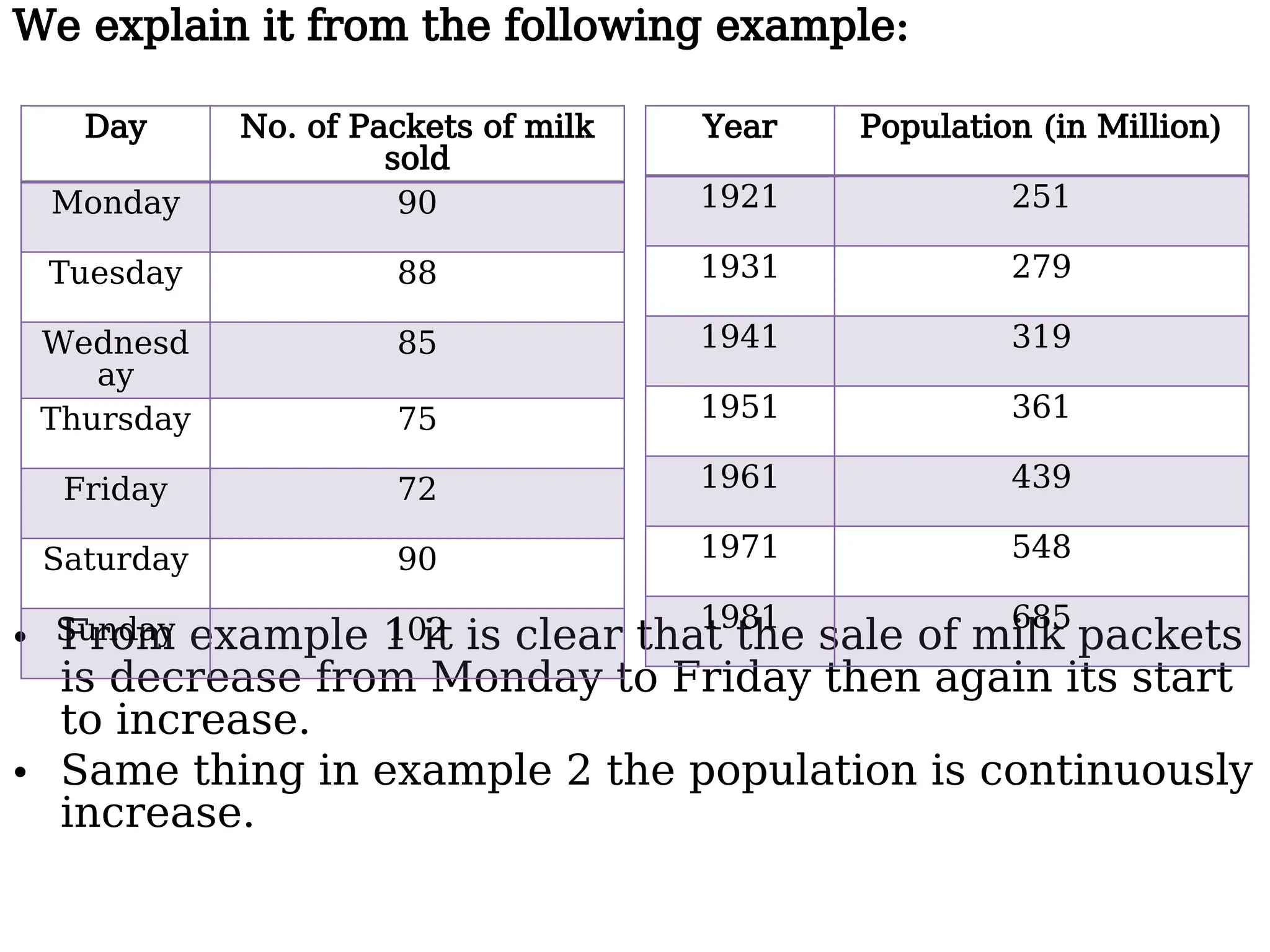
3. We explain it from the following example:
• From example 1 it is clear that the sale of milk packets
is decrease from Monday to Friday then again its start
to increase.
• Same thing in example 2 the population is continuously
increase.
Day No. of Packets of milk
sold
Monday 90
Tuesday 88
Wednesd
ay
85
Thursday 75
Friday 72
Saturday 90
Sunday 102
Year Population (in Million)
1921 251
1931 279
1941 319
1951 361
1961 439
1971 548
1981 685

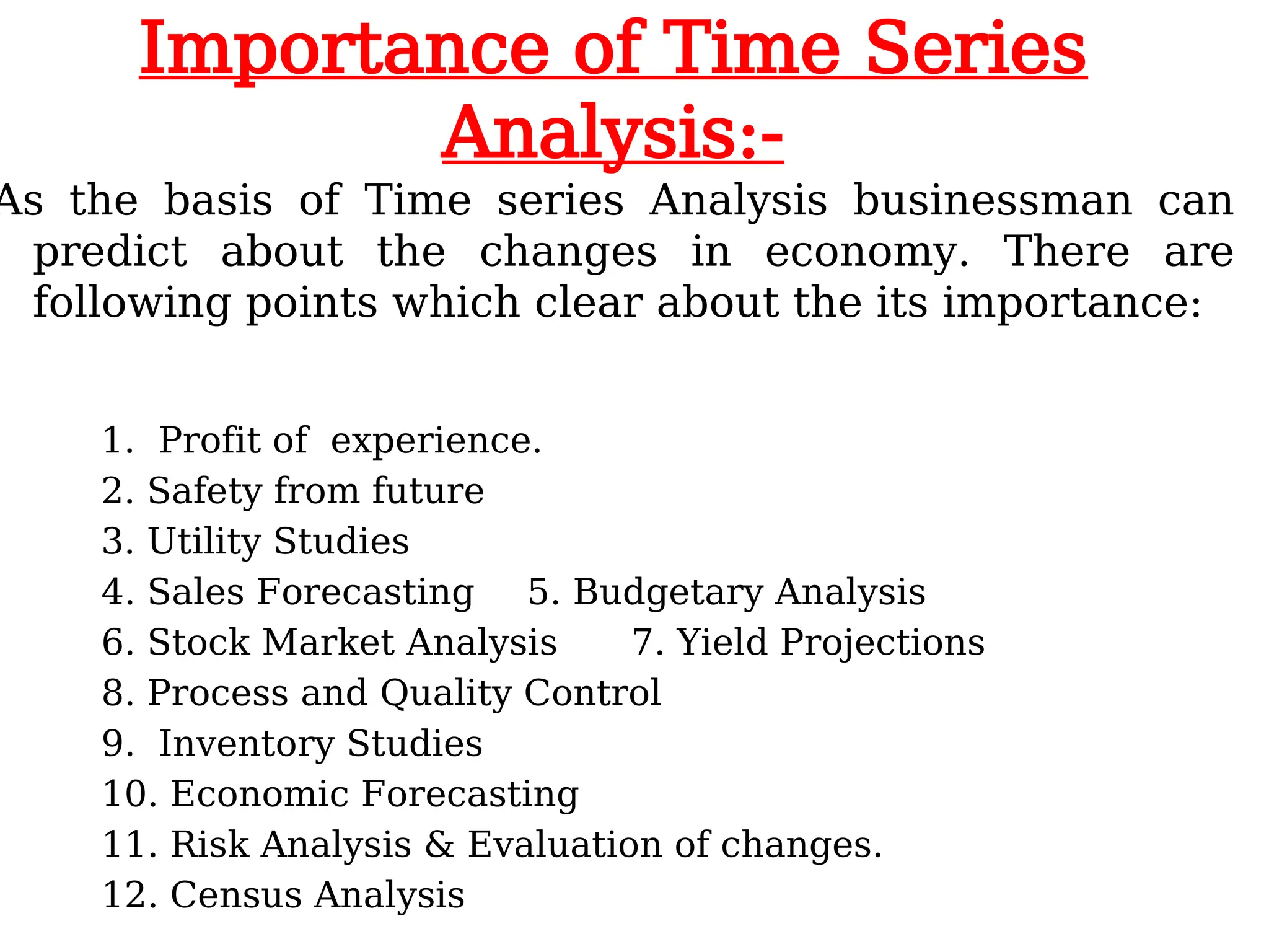
4. Importance of Time Series
Analysis:-
As the basis of Time series Analysis businessman can
predict about the changes in economy. There are
following points which clear about the its importance:
1. Profit of experience.
2. Safety from future
3. Utility Studies
4. Sales Forecasting 5. Budgetary Analysis
6. Stock Market Analysis 7. Yield Projections
8. Process and Quality Control
9. Inventory Studies
10. Economic Forecasting
11. Risk Analysis & Evaluation of changes.
12. Census Analysis

5. Components of Time Series:-
The change which are being in time series, They
are effected by Economic, Social, Natural,
Industrial & Political Reasons. These reasons
are called components of Time Series.
 Secular trend :-
 Seasonal variation :-
 Cyclical variation :-
 Irregular variation :-

6. 
Secular trend:
The increase or decrease in the movements of a time series
is called Secular trend.
A time series data may show upward trend or downward trend
for a period of years and this may be due to factors like:
 increase in population,
 change in technological progress ,
 large scale shift in consumers demands,
For example,
• population increases over a period of time,price increases
over a period of years,production of goods on the capital
market of the country increases over a period of years.These
are the examples of upward trend.
• The sales of a commodity may decrease over a period of time
because of better products coming to the market.This is an
example of declining trend or downward.

7. • Seasonal variation:
• Seasonal variation are short-term
fluctuation in a time series which occur
periodically in a year. This continues to
repeat year after year.
– The major factors that are weather
conditions and customs of people.
– More woolen clothes are sold in winter than
in the season of summer .
– each year more ice creams are sold in
summer and very little in Winter season.
– The sales in the departmental stores are
more during festive seasons that in the
normal days.

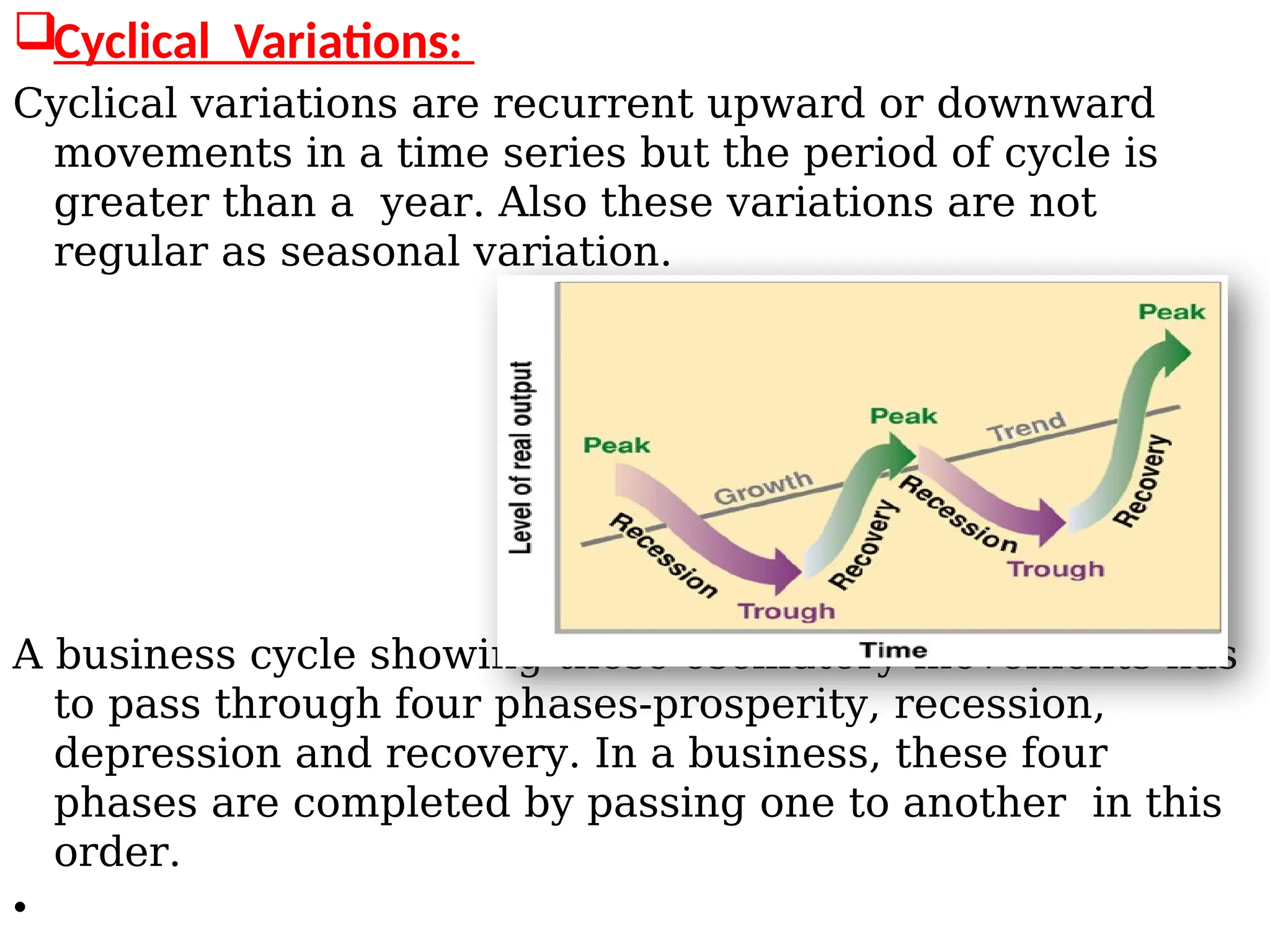
8. Cyclical Variations:
Cyclical variations are recurrent upward or downward
movements in a time series but the period of cycle is
greater than a year. Also these variations are not
regular as seasonal variation.
A business cycle showing these oscillatory movements has
to pass through four phases-prosperity, recession,
depression and recovery. In a business, these four
phases are completed by passing one to another in this
order.
•

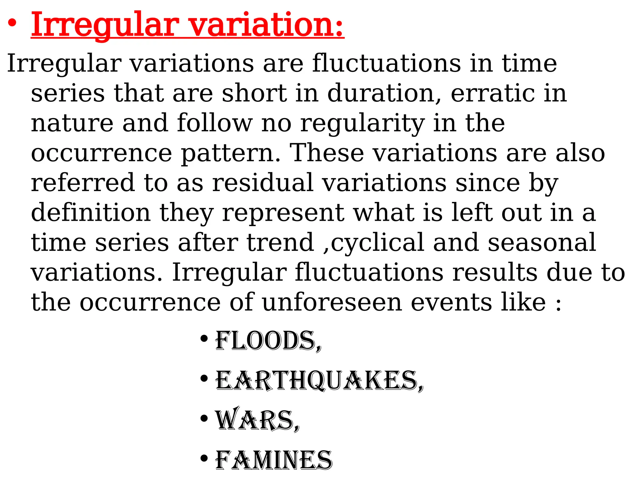
9. • Irregular variation:
Irregular variations are fluctuations in time
series that are short in duration, erratic in
nature and follow no regularity in the
occurrence pattern. These variations are also
referred to as residual variations since by
definition they represent what is left out in a
time series after trend ,cyclical and seasonal
variations. Irregular fluctuations results due to
the occurrence of unforeseen events like :
• Floods,
• Earthquakes,
• Wars,
• Famines

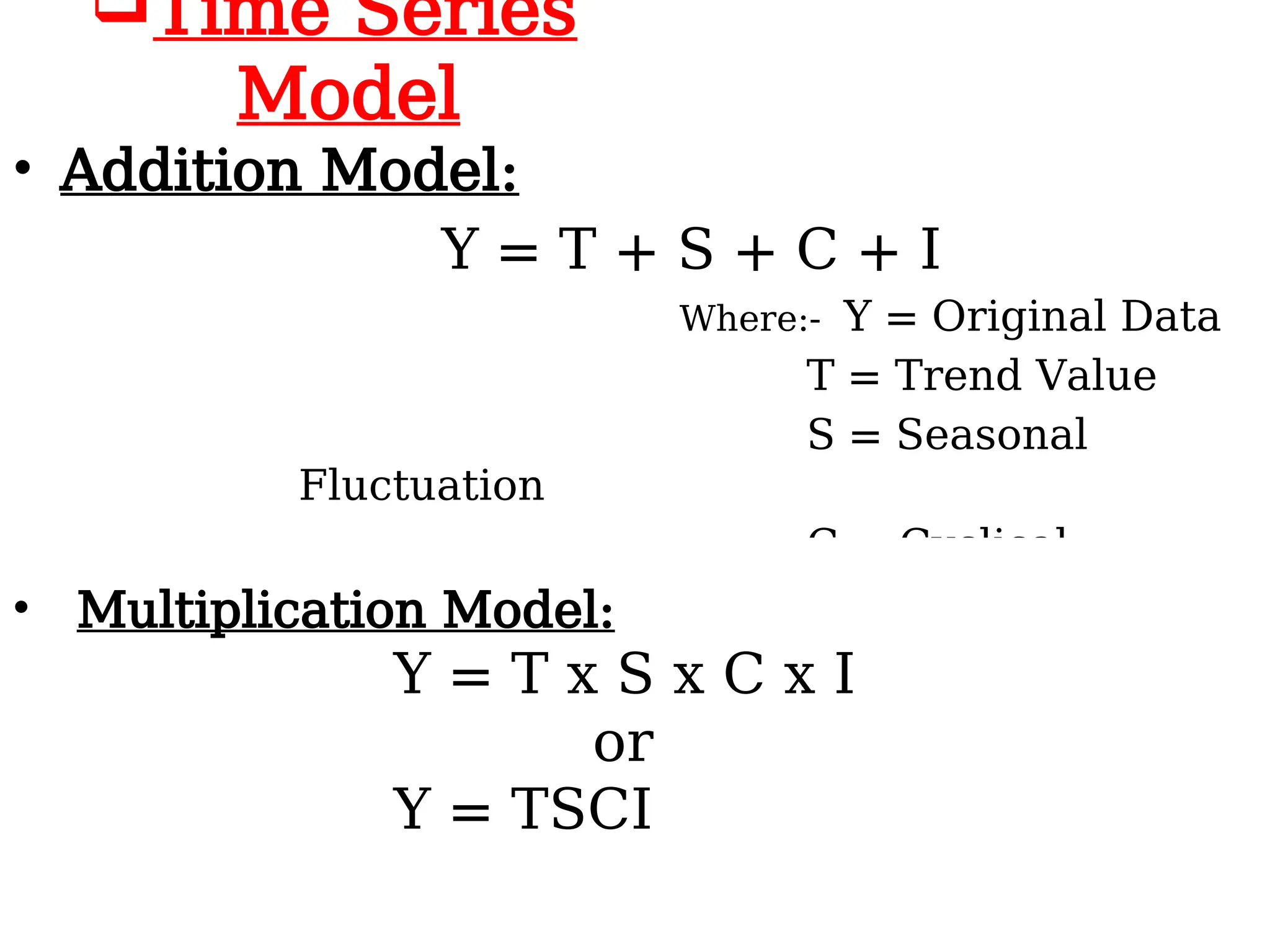
10. Time Series
Model
• Addition Model:
Y = T + S + C + I
Where:- Y = Original Data
T = Trend Value
S = Seasonal
Fluctuation
C = Cyclical
Fluctuation
I =
I = Irregular
Fluctuation
• Multiplication Model:
Y = T x S x C x I
or
Y = TSCI

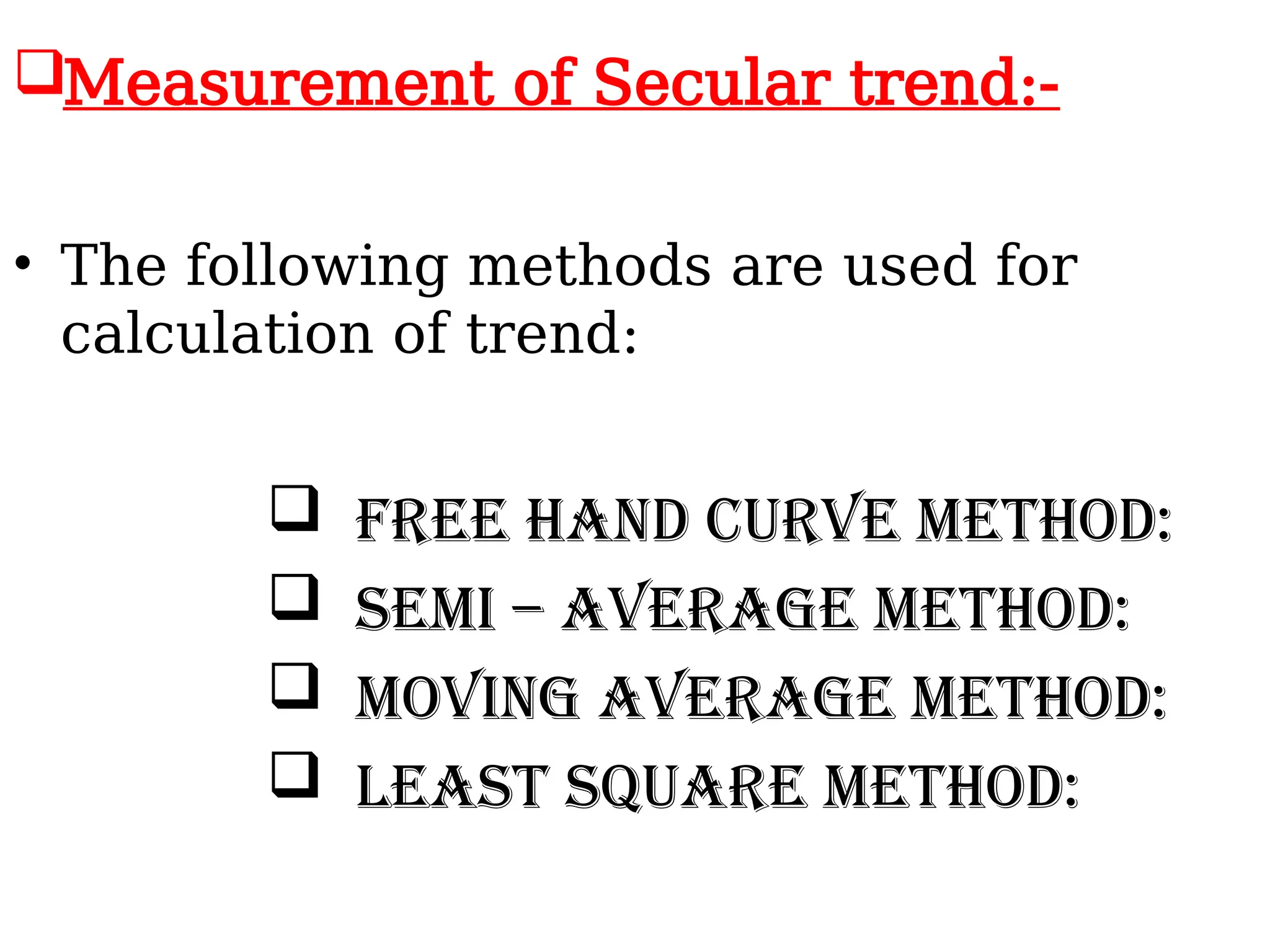
11. Measurement of Secular trend:-
• The following methods are used for
calculation of trend:
 Free Hand Curve Method:
 Semi – Average Method:
 Moving Average Method:
 Least Square Method:

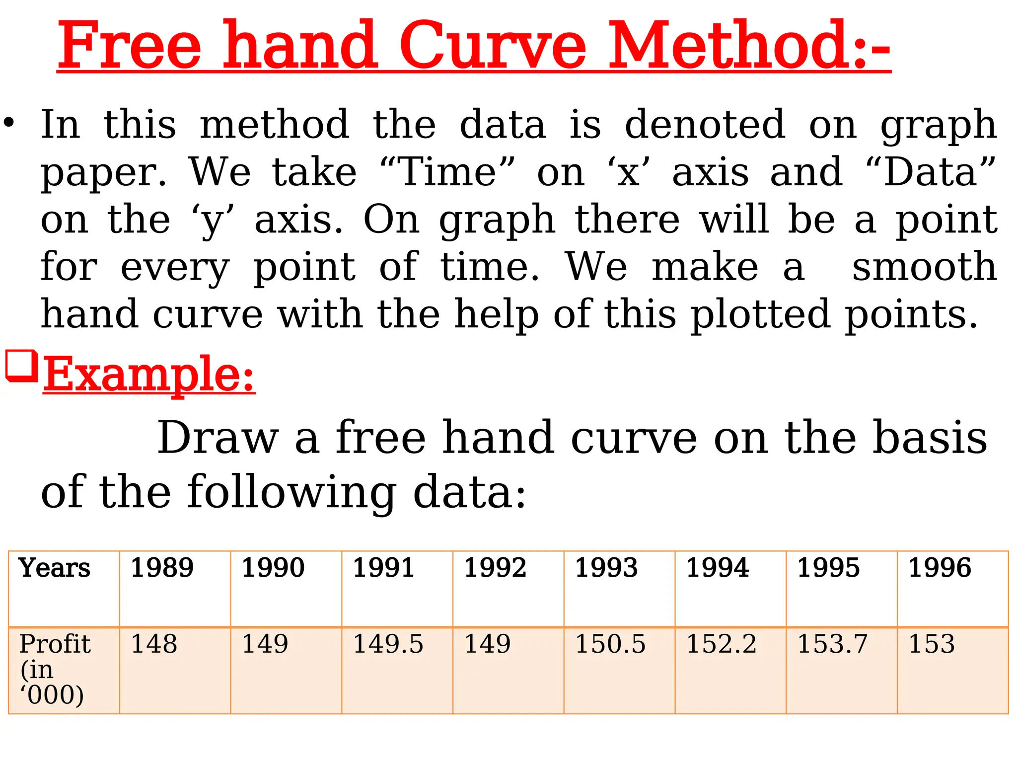
12. Free hand Curve Method:-
• In this method the data is denoted on graph
paper. We take “Time” on ‘x’ axis and “Data”
on the ‘y’ axis. On graph there will be a point
for every point of time. We make a smooth
hand curve with the help of this plotted points.
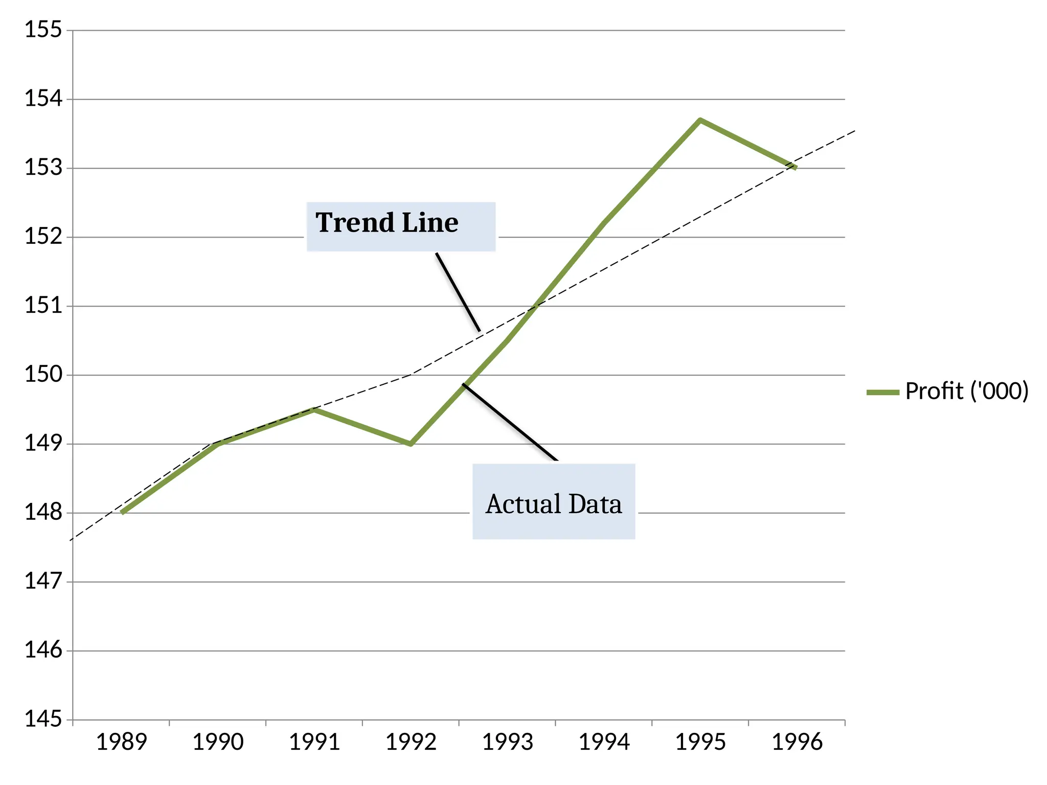
Example:
Draw a free hand curve on the basis
of the following data:
Years 1989 1990 1991 1992 1993 1994 1995 1996
Profit
(in
‘000)
148 149 149.5 149 150.5 152.2 153.7 153

13. 1989 1990 1991 1992 1993 1994 1995 1996
145
146
147
148
149
150
151
152
153
154
155
Profit ('000)
Trend Line
Actual Data

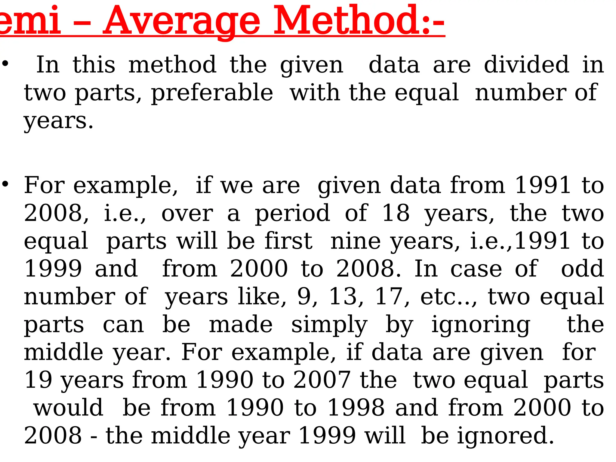
14. emi – Average Method:-
• In this method the given data are divided in
two parts, preferable with the equal number of
years.
• For example, if we are given data from 1991 to
2008, i.e., over a period of 18 years, the two
equal parts will be first nine years, i.e.,1991 to
1999 and from 2000 to 2008. In case of odd
number of years like, 9, 13, 17, etc.., two equal
parts can be made simply by ignoring the
middle year. For example, if data are given for
19 years from 1990 to 2007 the two equal parts
would be from 1990 to 1998 and from 2000 to
2008 - the middle year 1999 will be ignored.

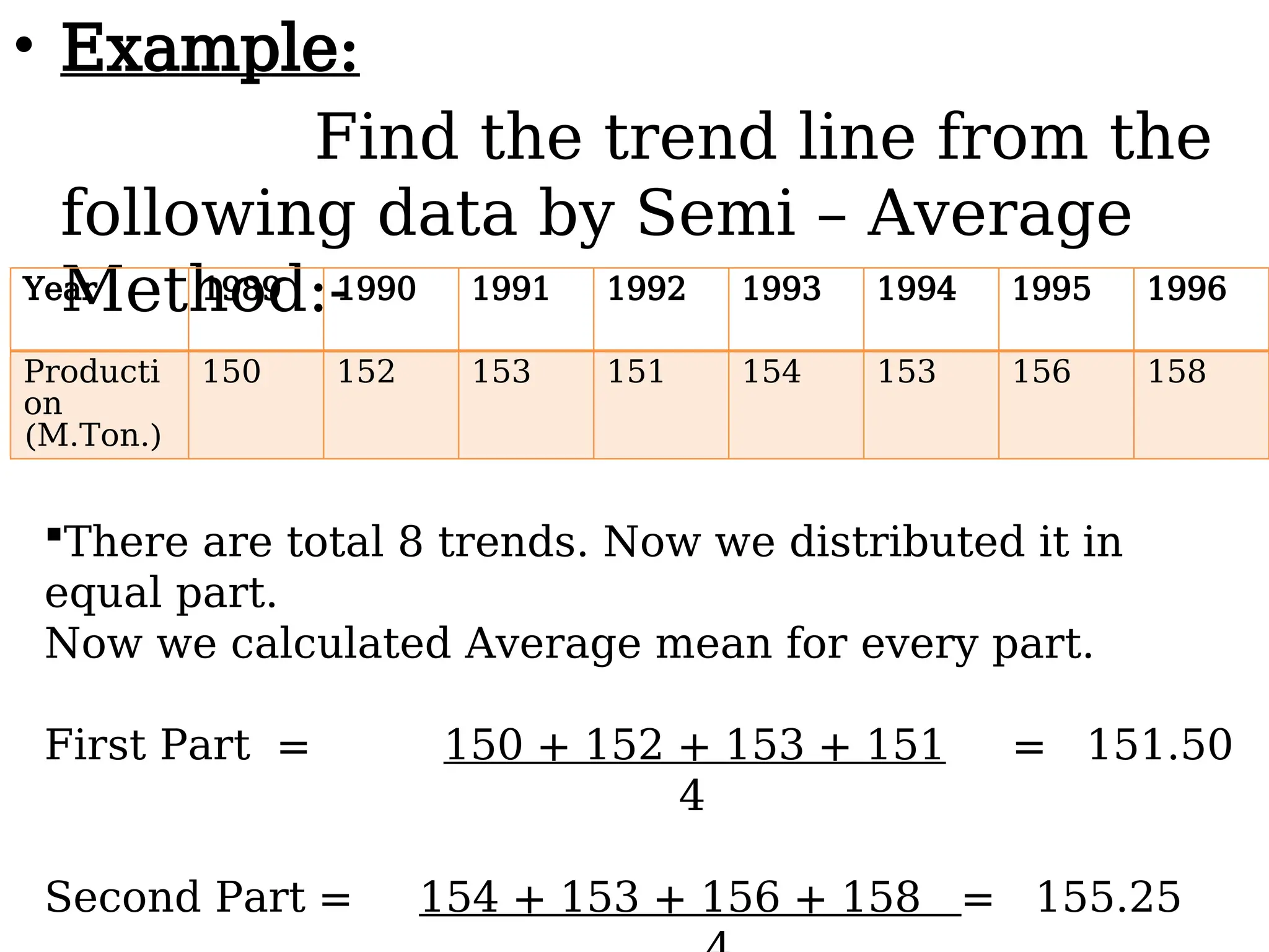
15. • Example:
Find the trend line from the
following data by Semi – Average
Method:-
Year 1989 1990 1991 1992 1993 1994 1995 1996
Producti
on
(M.Ton.)
150 152 153 151 154 153 156 158
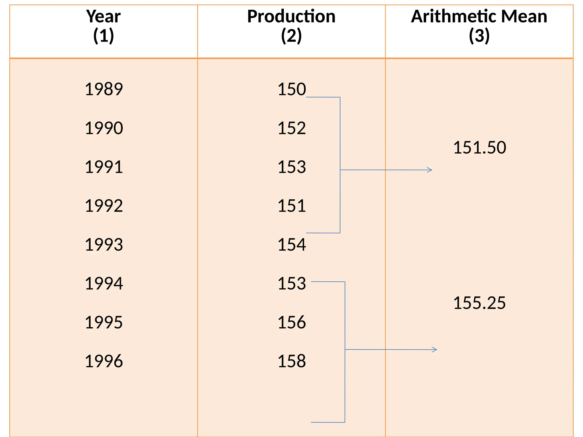
There are total 8 trends. Now we distributed it in
equal part.
Now we calculated Average mean for every part.
First Part = 150 + 152 + 153 + 151 = 151.50
4
Second Part = 154 + 153 + 156 + 158 = 155.25

16. Year
(1)
Production
(2)
Arithmetic Mean
(3)
1989
1990
1991
1992
1993
1994
1995
1996
150
152
153
151
154
153
156
158
151.50
155.25

17. 1989 1990 1991 1992 1993 1994 1995 1996
146
148
150
152
154
156
158
160
Production
Production
151.50
155.25

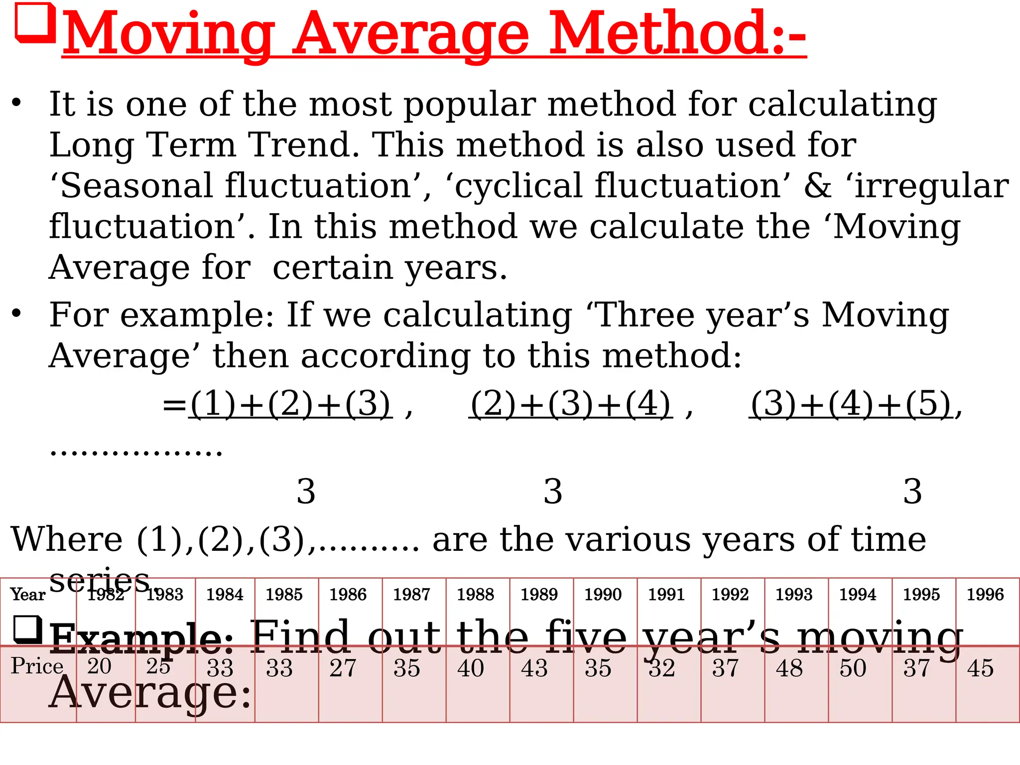
18. Moving Average Method:-
• It is one of the most popular method for calculating
Long Term Trend. This method is also used for
‘Seasonal fluctuation’, ‘cyclical fluctuation’ & ‘irregular
fluctuation’. In this method we calculate the ‘Moving
Average for certain years.
• For example: If we calculating ‘Three year’s Moving
Average’ then according to this method:
=(1)+(2)+(3) , (2)+(3)+(4) , (3)+(4)+(5),
……………..
3 3 3
Where (1),(2),(3),………. are the various years of time
series.
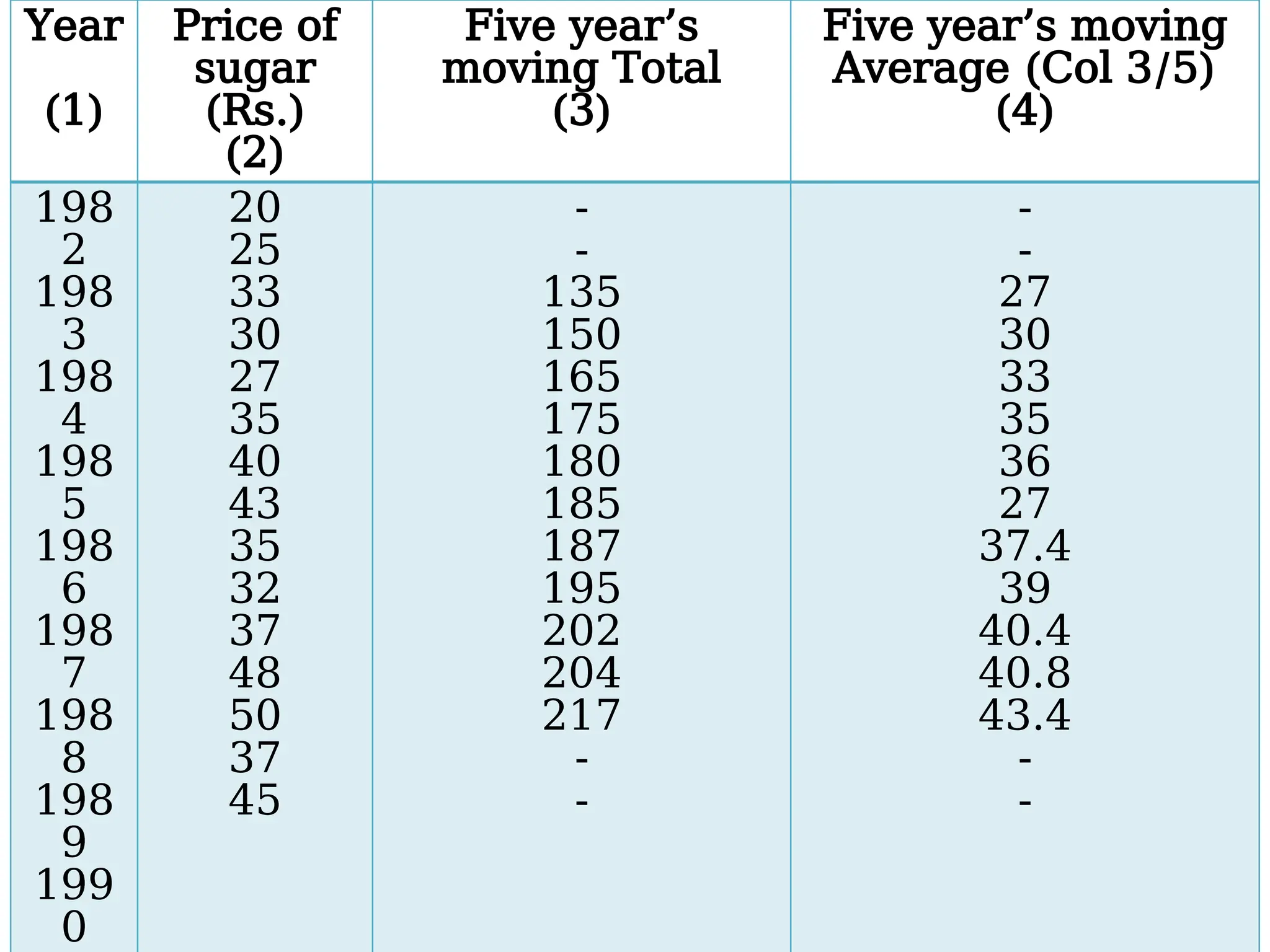
Example: Find out the five year’s moving
Average:
Year 1982 1983 1984 1985 1986 1987 1988 1989 1990 1991 1992 1993 1994 1995 1996
Price 20 25 33 33 27 35 40 43 35 32 37 48 50 37 45

19. Year
(1)
Price of
sugar
(Rs.)
(2)
Five year’s
moving Total
(3)
Five year’s moving
Average (Col 3/5)
(4)
198
2
198
3
198
4
198
5
198
6
198
7
198
8
198
9
199
0
20
25
33
30
27
35
40
43
35
32
37
48
50
37
45
-
-
135
150
165
175
180
185
187
195
202
204
217
-
-
-
-
27
30
33
35
36
27
37.4
39
40.4
40.8
43.4
-
-

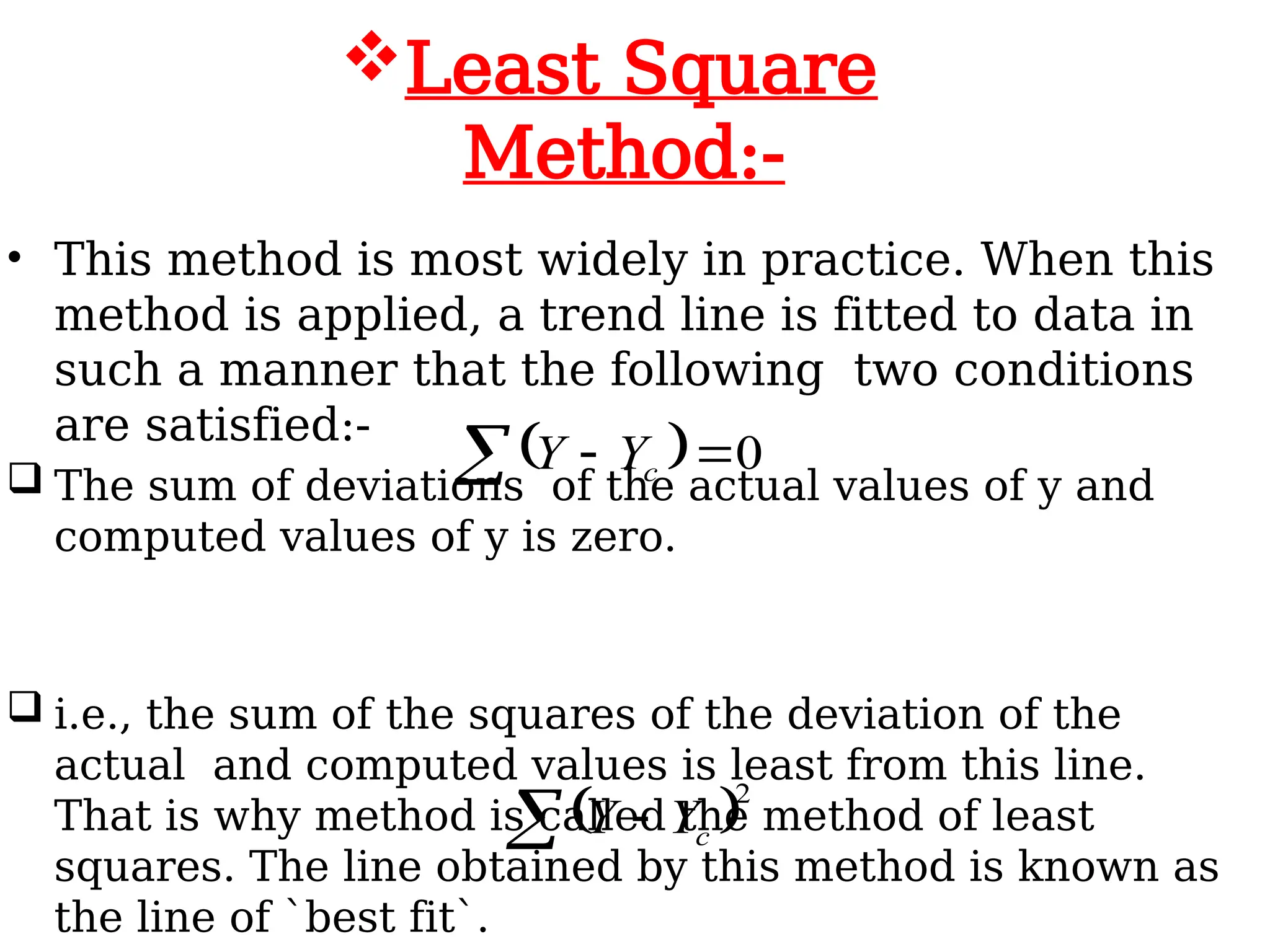
20. • This method is most widely in practice. When this
method is applied, a trend line is fitted to data in
such a manner that the following two conditions
are satisfied:-
 The sum of deviations of the actual values of y and
computed values of y is zero.
 i.e., the sum of the squares of the deviation of the
actual and computed values is least from this line.
That is why method is called the method of least
squares. The line obtained by this method is known as
the line of `best fit`.
Least Square
Method:-
  0


 c
Y
Y
 2
  c
Y
Y

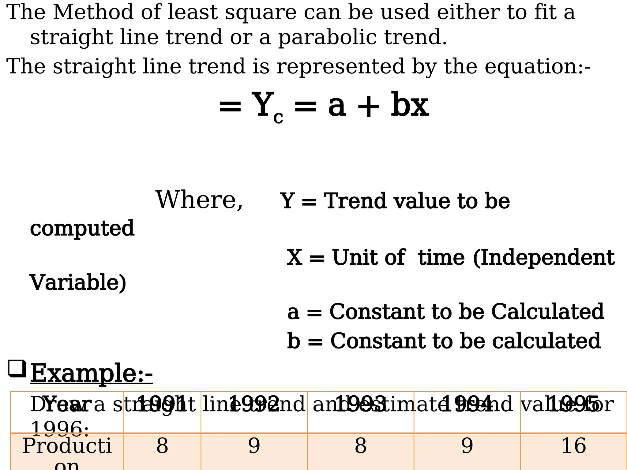
21. The Method of least square can be used either to fit a
straight line trend or a parabolic trend.
The straight line trend is represented by the equation:-
= Yc = a + bx
Where, Y = Trend value to be
computed
X = Unit of time (Independent
Variable)
a = Constant to be Calculated
b = Constant to be calculated
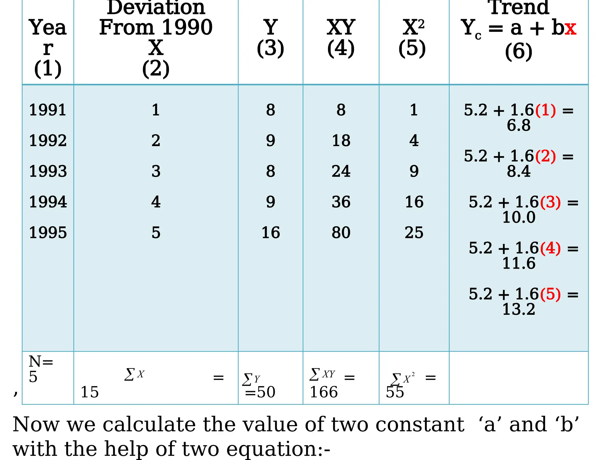
Example:-
Draw a straight line trend and estimate trend value for
1996:
Year 1991 1992 1993 1994 1995
Producti 8 9 8 9 16

22. Yea
r
(1)
Deviation
From 1990
X
(2)
Y
(3)
XY
(4)
X2
(5)
Trend
Yc = a + bx
(6)
1991
1992
1993
1994
1995
1
2
3
4
5
8
9
8
9
16
8
18
24
36
80
1
4
9
16
25
5.2 + 1.6(1) =
6.8
5.2 + 1.6(2) =
8.4
5.2 + 1.6(3) =
10.0
5.2 + 1.6(4) =
11.6
5.2 + 1.6(5) =
13.2
N=
5 =
15 =50
=
166
=
55
 X
Y  XY 2
 X
’
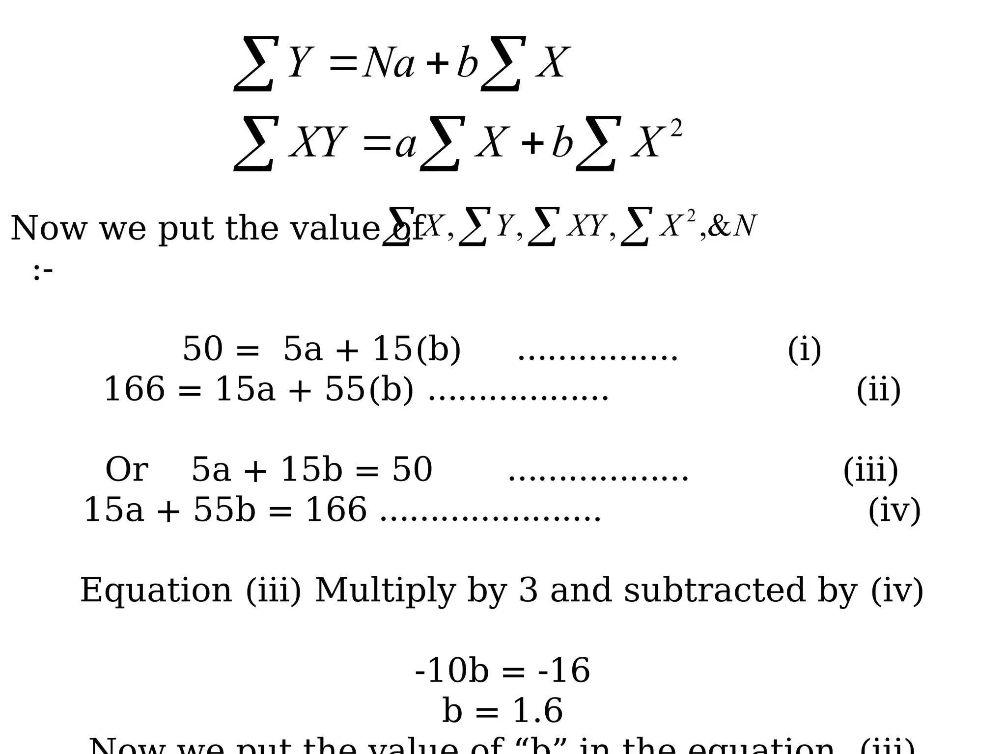
Now we calculate the value of two constant ‘a’ and ‘b’
with the help of two equation:-

23.   
 




2
X
b
X
a
XY
X
b
Na
Y
Now we put the value of
:-
50 = 5a + 15(b) ……………. (i)
166 = 15a + 55(b) ……………… (ii)
Or 5a + 15b = 50 ……………… (iii)
15a + 55b = 166 …………………. (iv)
Equation (iii) Multiply by 3 and subtracted by (iv)
-10b = -16
b = 1.6
    N
X
XY
Y
X ,&
,
,
, 2

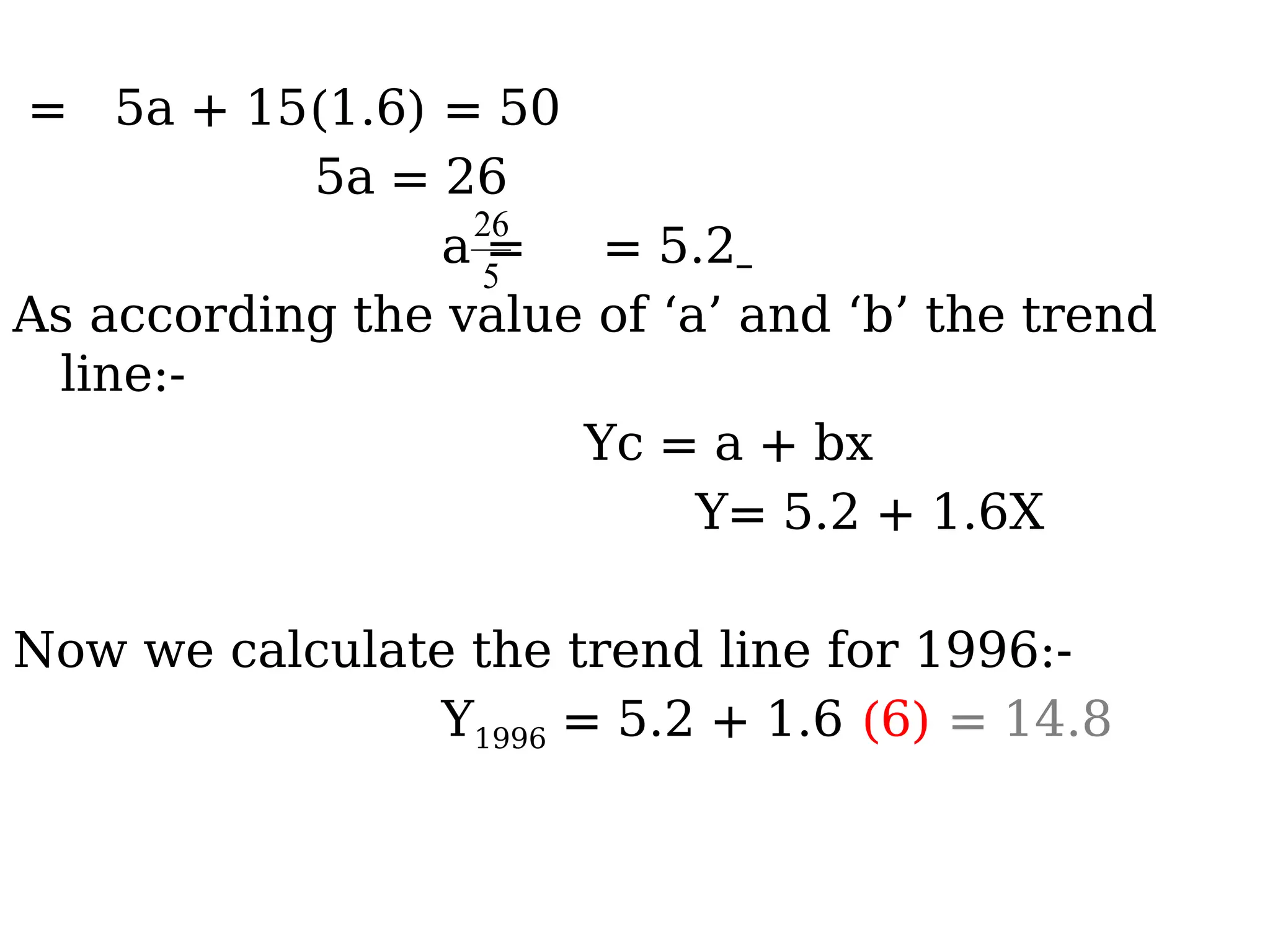
24. = 5a + 15(1.6) = 50
5a = 26
a = = 5.2
As according the value of ‘a’ and ‘b’ the trend
line:-
Yc = a + bx
Y= 5.2 + 1.6X
Now we calculate the trend line for 1996:-
Y1996 = 5.2 + 1.6 (6) = 14.8
5
26

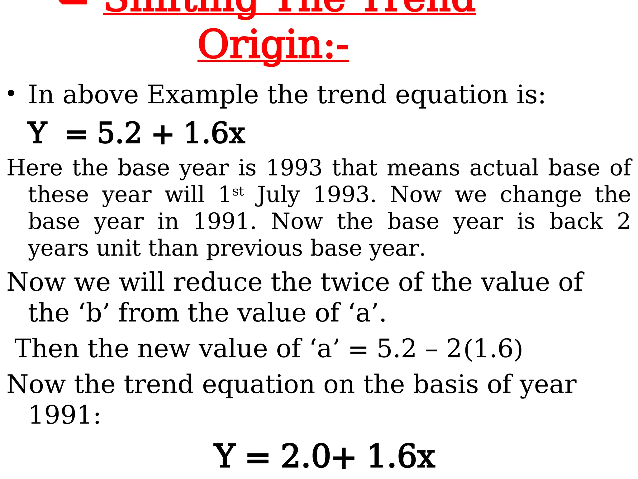
25.  Shifting The Trend
Origin:-
• In above Example the trend equation is:
Y = 5.2 + 1.6x
Here the base year is 1993 that means actual base of
these year will 1st
July 1993. Now we change the
base year in 1991. Now the base year is back 2
years unit than previous base year.
Now we will reduce the twice of the value of
the ‘b’ from the value of ‘a’.
Then the new value of ‘a’ = 5.2 – 2(1.6)
Now the trend equation on the basis of year
1991:
Y = 2.0+ 1.6x

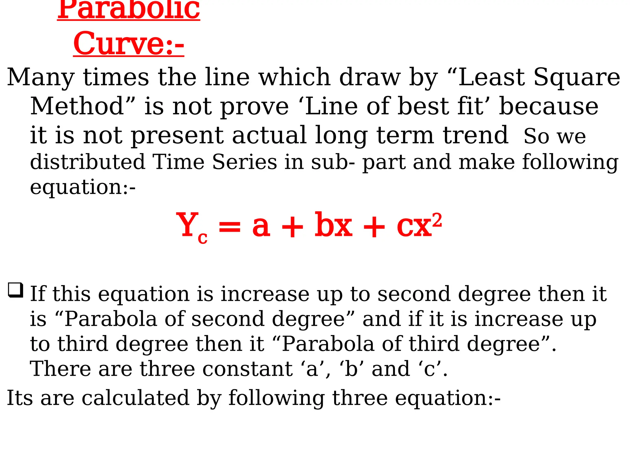
26. Parabolic
Curve:-
Many times the line which draw by “Least Square
Method” is not prove ‘Line of best fit’ because
it is not present actual long term trend So we
distributed Time Series in sub- part and make following
equation:-
Yc = a + bx + cx2
 If this equation is increase up to second degree then it
is “Parabola of second degree” and if it is increase up
to third degree then it “Parabola of third degree”.
There are three constant ‘a’, ‘b’ and ‘c’.
Its are calculated by following three equation:-

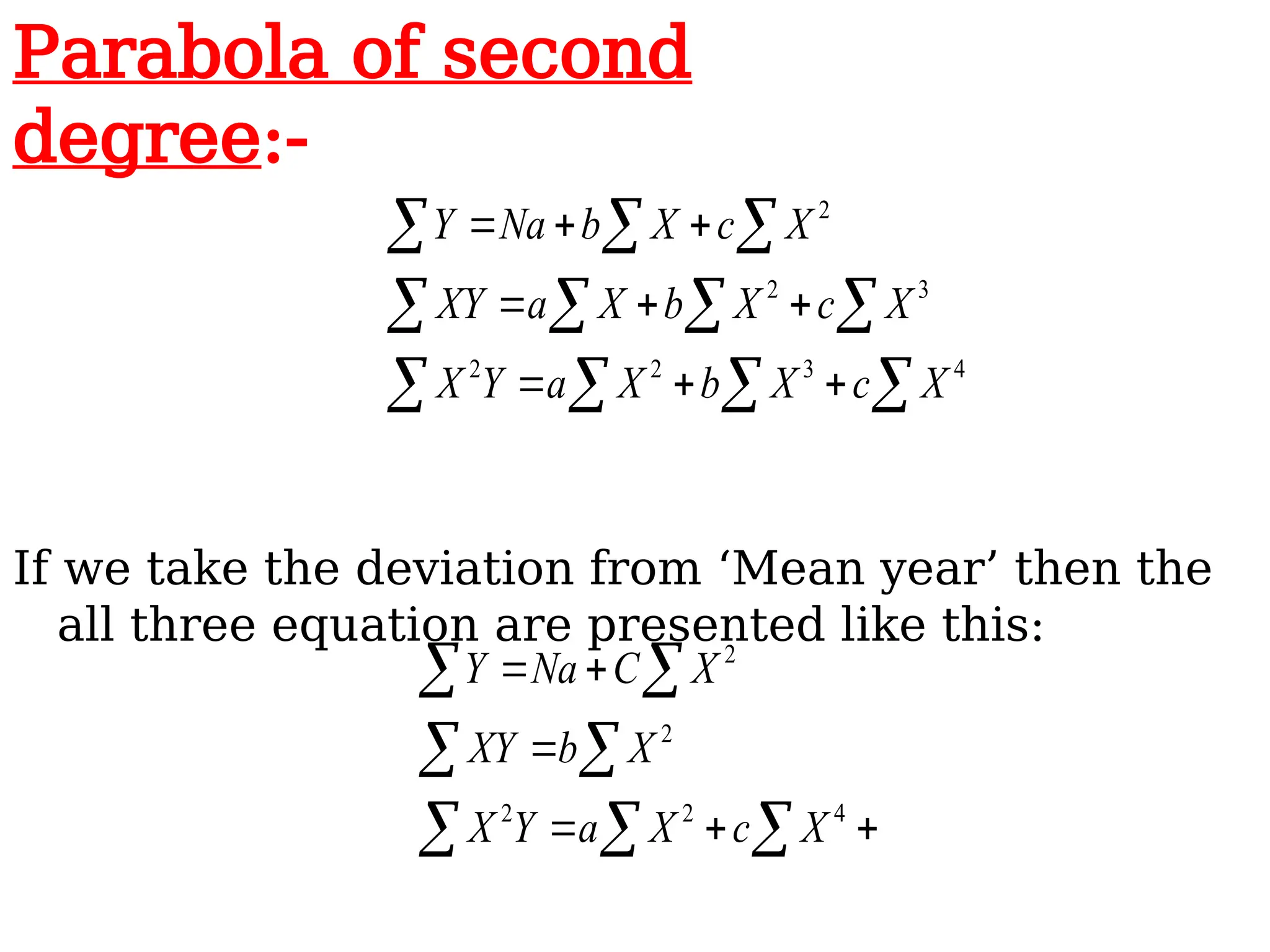
27. If we take the deviation from ‘Mean year’ then the
all three equation are presented like this:
  
 
 






4
2
2
2
2
X
c
X
a
Y
X
X
b
XY
X
C
Na
Y
  

  

  









4
3
2
2
3
2
2
X
c
X
b
X
a
Y
X
X
c
X
b
X
a
XY
X
c
X
b
Na
Y
Parabola of second
degree:-

28. Yea
r
Productio
n
Dev. From
Middle
Year
(x)
xY x2
x2
Y x3
x4
Trend Value
Y = a + bx +
cx2
1992
1993
1994
1995
1996
5
7
4
9
10
-2
-1
0
1
2
-10
-7
0
9
20
4
1
0
1
4
20
7
0
9
40
-8
-1
0
1
8
16
1
0
1
16
5.7
5.6
6.3
8.0
10.5
= 35 = 0 =12 = 10 = 76 = 0 = 34
Y  X  XY  2
X Y
X
 2
 3
X  4
X
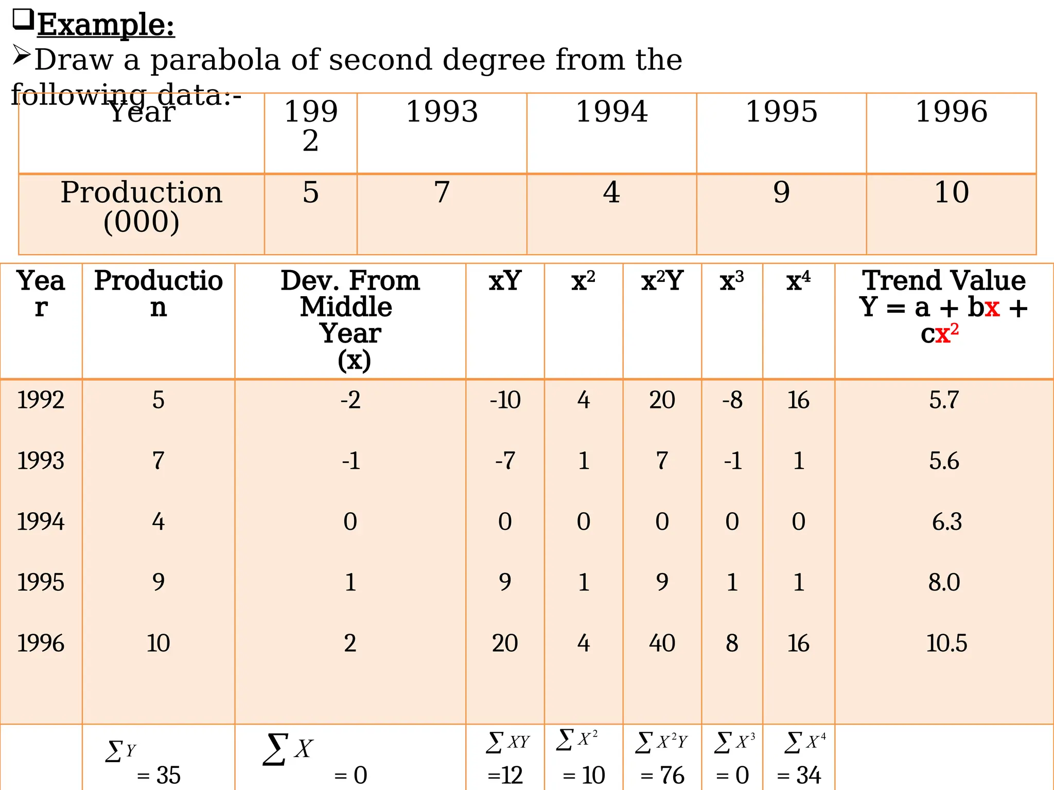
Example:
Draw a parabola of second degree from the
following data:-
Year 199
2
1993 1994 1995 1996
Production
(000)
5 7 4 9 10

29.   
 
 






4
2
2
2
2
X
c
X
a
Y
X
X
b
XY
X
Na
Y
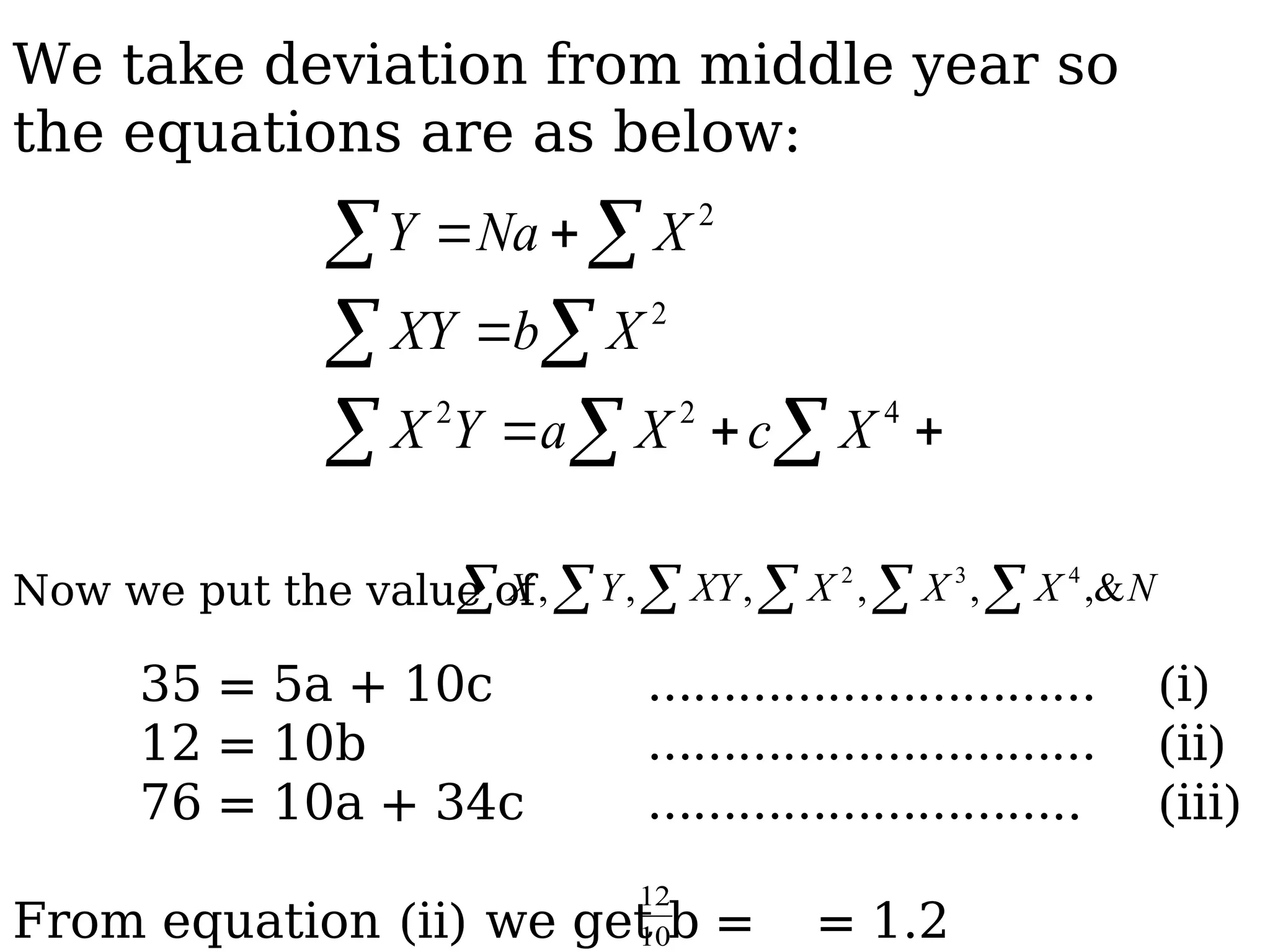
Now we put the value of
35 = 5a + 10c ………………………… (i)
12 = 10b ………………………… (ii)
76 = 10a + 34c ……………………….. (iii)
From equation (ii) we get b = = 1.2
   

 N
X
X
X
XY
Y
X ,&
,
,
,
,
, 4
3
2
10
12
We take deviation from middle year so
the equations are as below:

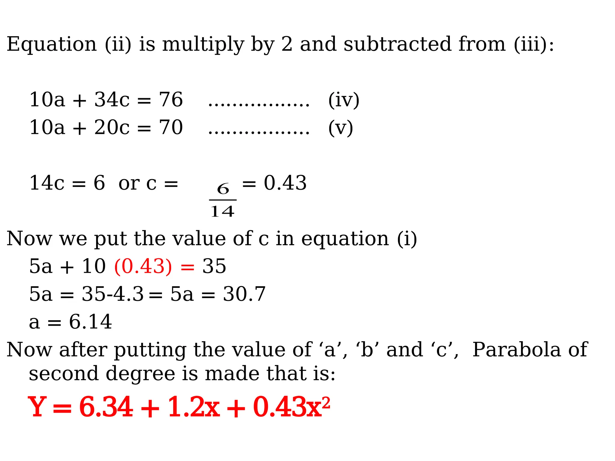
30. Equation (ii) is multiply by 2 and subtracted from (iii):
10a + 34c = 76 …………….. (iv)
10a + 20c = 70 …………….. (v)
14c = 6 or c = = 0.43
Now we put the value of c in equation (i)
5a + 10 (0.43) = 35
5a = 35-4.3 = 5a = 30.7
a = 6.14
Now after putting the value of ‘a’, ‘b’ and ‘c’, Parabola of
second degree is made that is:
Y = 6.34 + 1.2x + 0.43x2
14
6

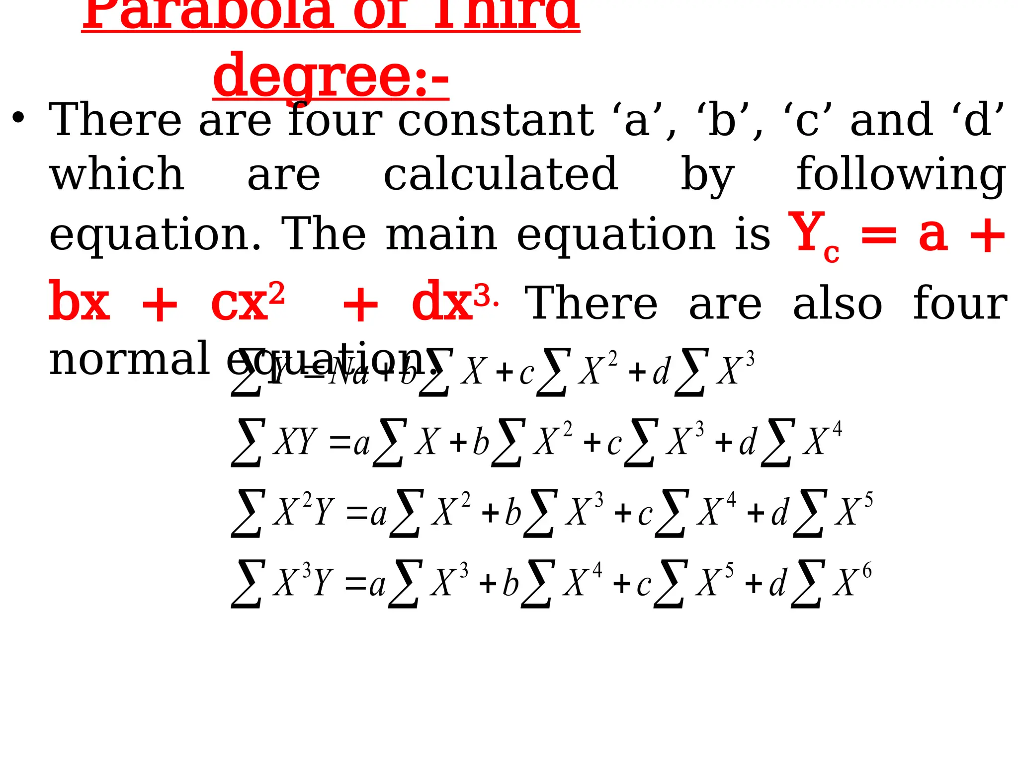
31. Parabola of Third
degree:-
• There are four constant ‘a’, ‘b’, ‘c’ and ‘d’
which are calculated by following
equation. The main equation is Yc = a +
bx + cx2
+ dx3. There are also four
normal equation.
  


  


   


  
















6
5
4
3
3
5
4
3
2
2
4
3
2
3
2
X
d
X
c
X
b
X
a
Y
X
X
d
X
c
X
b
X
a
Y
X
X
d
X
c
X
b
X
a
XY
X
d
X
c
X
b
Na
Y

32. Methods Of Seasonal
Variation:-
•Seasonal Average Method
•Link Relative Method
•Ratio To Trend Method
•Ratio To Moving Average Method

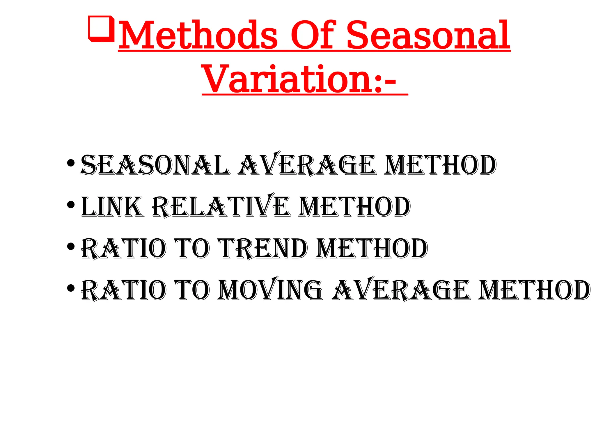
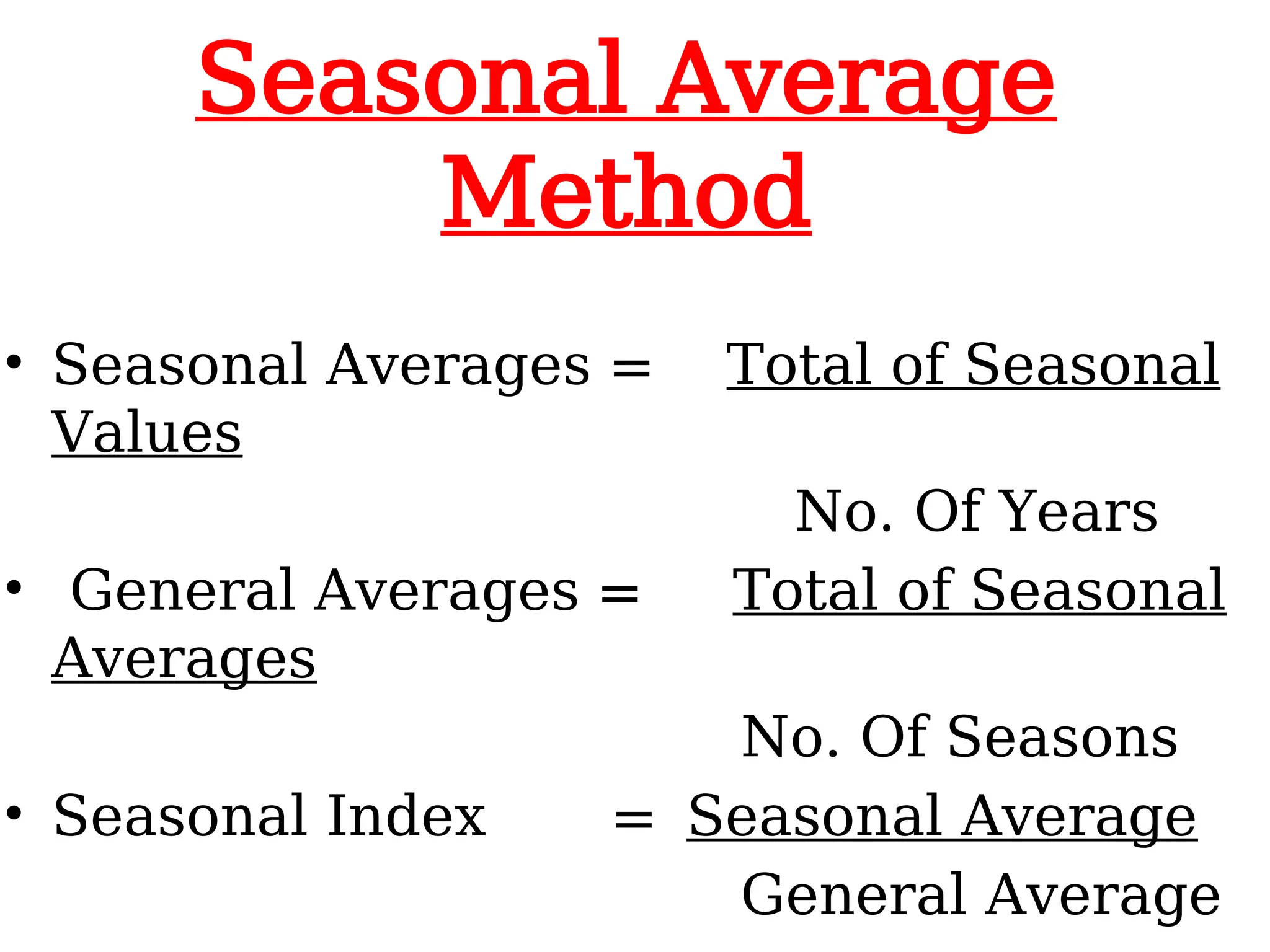
33. Seasonal Average
Method
• Seasonal Averages = Total of Seasonal
Values
No. Of Years
• General Averages = Total of Seasonal
Averages
No. Of Seasons
• Seasonal Index = Seasonal Average
General Average

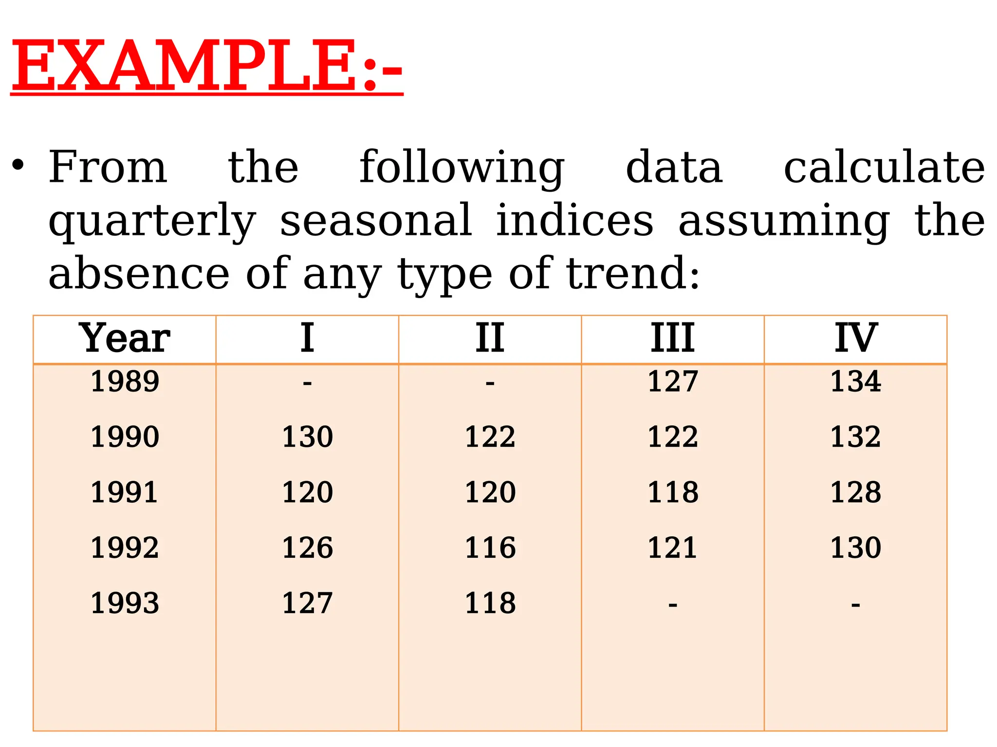
34. EXAMPLE:-
• From the following data calculate
quarterly seasonal indices assuming the
absence of any type of trend:
Year I II III IV
1989
1990
1991
1992
1993
-
130
120
126
127
-
122
120
116
118
127
122
118
121
-
134
132
128
130
-

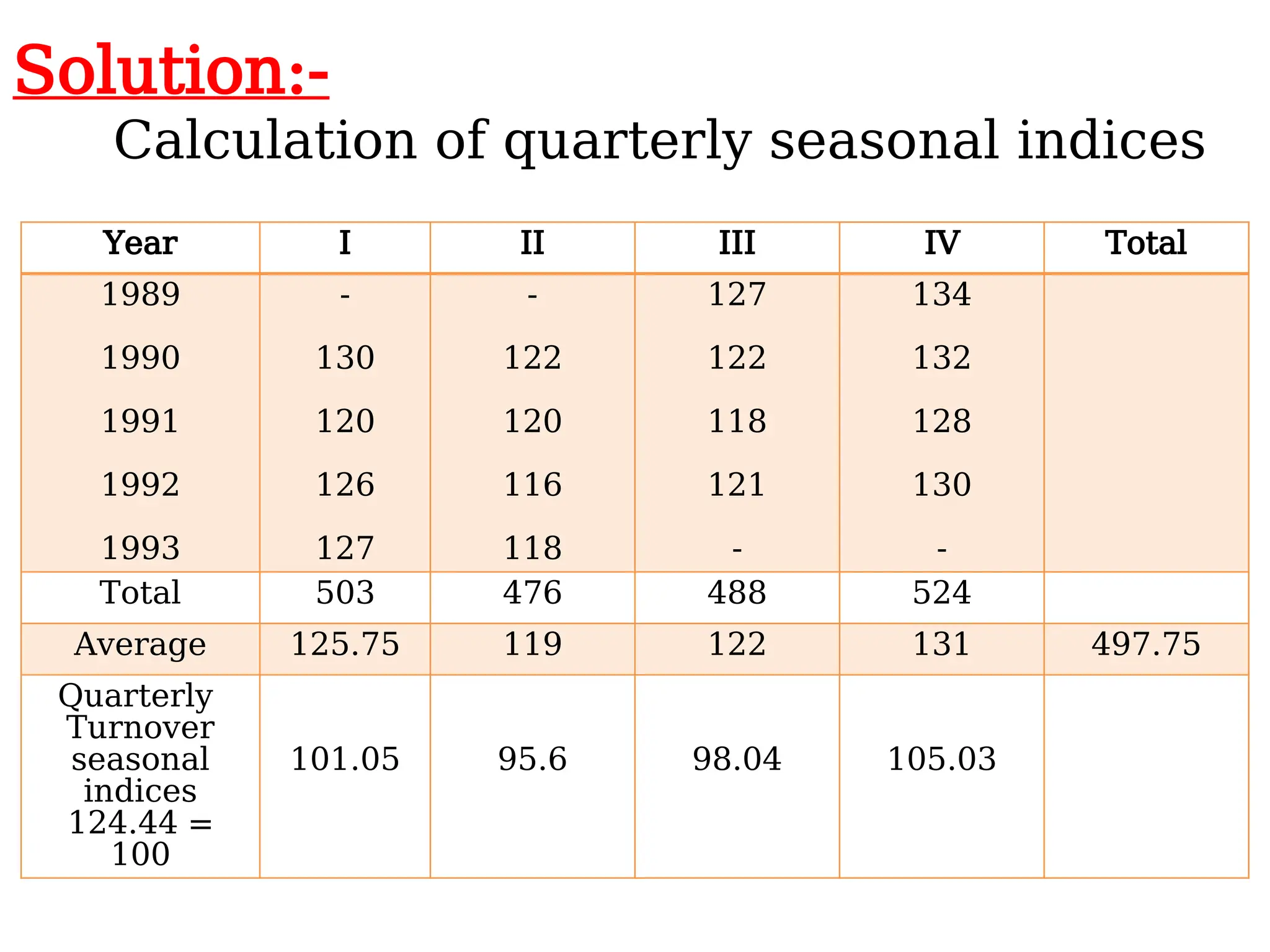
35. Solution:-
Calculation of quarterly seasonal indices
Year I II III IV Total
1989
1990
1991
1992
1993
-
130
120
126
127
-
122
120
116
118
127
122
118
121
-
134
132
128
130
-
Total 503 476 488 524
Average 125.75 119 122 131 497.75
Quarterly
Turnover
seasonal
indices
124.44 =
100
101.05 95.6 98.04 105.03

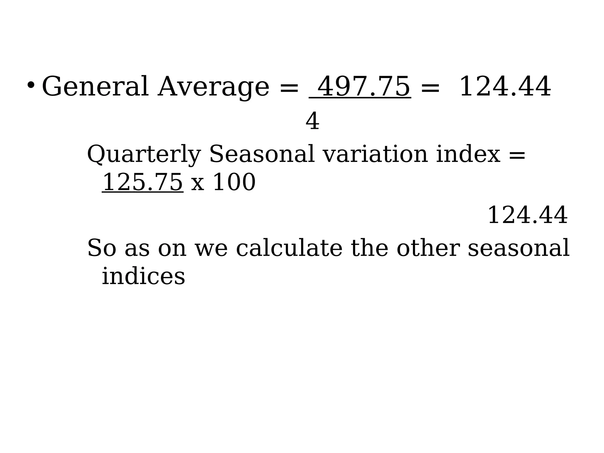
36. • General Average = 497.75 = 124.44
4
Quarterly Seasonal variation index =
125.75 x 100
124.44
So as on we calculate the other seasonal
indices

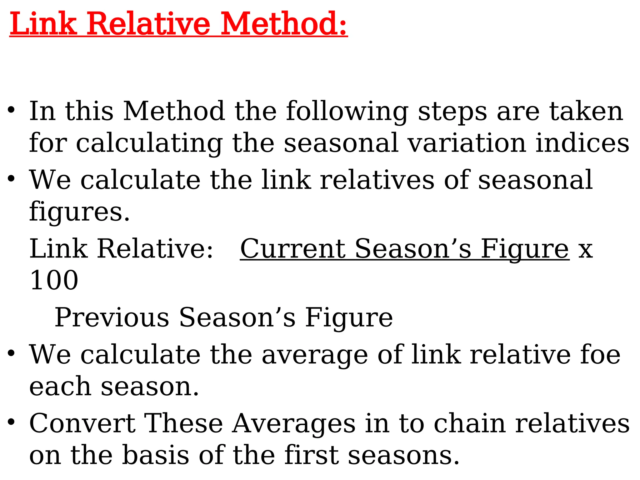
37. Link Relative Method:
• In this Method the following steps are taken
for calculating the seasonal variation indices
• We calculate the link relatives of seasonal
figures.
Link Relative: Current Season’s Figure x
100
Previous Season’s Figure
• We calculate the average of link relative foe
each season.
• Convert These Averages in to chain relatives
on the basis of the first seasons.

38. • Calculate the chain relatives of the first
season on the base of the last seasons.
There will be some difference between
the chain relatives of the first seasons
and the chain relatives calculated by the
pervious Method.
• This difference will be due to effect of
long term changes.
• For correction the chain relatives of the
first season calculated by 1st
method is
deducted from the chain relative
calculated by the second method.
• Then Express the corrected chain

39. Ratio To Moving Average
Method:
• In this method seasonal variation indices
are calculated in following steps:
• We calculate the 12 monthly or 4
quarterly moving average.
• We use following formula for calculating
the moving average Ratio:
Moving Average Ratio= Original
Data x 100
Moving Average
Then we calculate the seasonal variation

40. Ratio To Trend
Method:-
• This method based on Multiple model of Time
Series. In It We use the following Steps:
• We calculate the trend value for various time
duration (Monthly or Quarterly) with the help
of Least Square method
• Then we express the all original data as the
percentage of trend on the basis of the
following formula.
= Original Data x 100
Trend Value
Rest of Process are as same as moving Average
Method

41. Methods Of Cyclical
Variation:-
Residual Method
References cycle analysis
method
Direct Method
Harmonic Analysis Method

42. Residual Method:-
• Cyclical variations are calculated by Residual Method . This
method is based on the multiple model of the time Series. The
process is as below:
• (a) When yearly data are given:
In class of yearly data there are not any seasonal variations so
original data are effect by three components:
• Trend Value
• Cyclical
• Irregular
First we calculate the seasonal variation indices according to moving
average ratio method.
At last we express the cyclical and irregular variation as the Trend
Ratio & Seasonal variation Indices
(b) When monthly or quarterly data are
given:

43. Measurement of Irregular
Variations
• The irregular components in a time
series represent the residue of
fluctuations after trend cycle and
seasonal movements have been
accounted for. Thus if the original data is
divided by T,S and C ; we get I i.e. . In
Practice the cycle itself is so erratic and
is so interwoven with irregular
movement that is impossible to separate

44. References:-
• Books of Business Statistics S.P.Gupta &
M.P.Gupta
• Books of Business Statistics :
Mathur, Khandelwal,
Gupta & Gupta

45. m