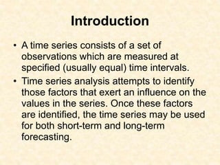
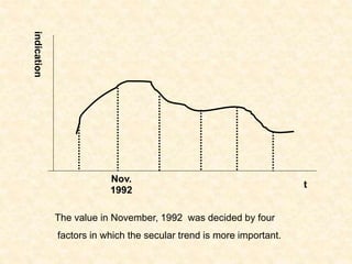
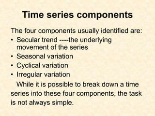
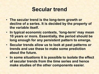
This document discusses various methods for analyzing time series data and identifying trends, including: 1. A time series consists of observations measured at regular intervals, and time series analysis aims to identify influencing factors to allow for forecasting. 2. The four main components of variations in time series are secular trends, seasonal variations, cyclical variations, and irregular variations. 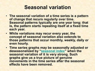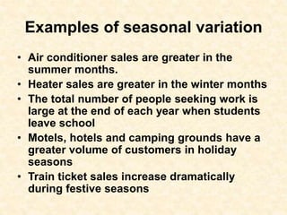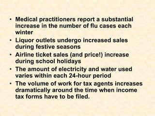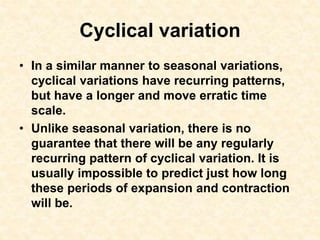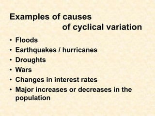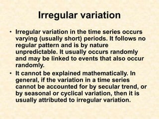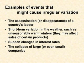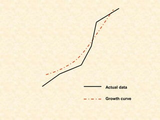3. Secular trends represent long-term growth or decline, while seasonal variations have annual patterns. Cyclical variations have less predictable recurring patterns, and irregular variations occur randomly.

1. Topic11: Time series and trend analysis
060074
STATISTICS

2. Introduction
• A time series consists of a set of
observations which are measured at
specified (usually equal) time intervals.
• Time series analysis attempts to identify
those factors that exert an influence on the
values in the series. Once these factors
are identified, the time series may be used
for both short-term and long-term
forecasting.

3. A several of time series
year
GDP
(100 million
yuan)
Total
population
(year-end)
(10000
persons)
Natural Growth
Rate of
Population
(‰)
Household
consumption
expenditures
(yuan)
2001
2002
2003
2004
2005
2006
2007
2008
2009
2010
18547.9
21617.8
26638.1
34634.4
46759.4
58478.1
67884.6
74772.4
79552.8
80471.6
114333
115823
117171
118517
119850
121121
122389
123626
124810
125924
14.39
12.98
11.60
11.45
11.21
10.55
10.42
10.06
9.53
9.48
803
896
1070
1331
1781
2311
2726
2944
3094
3130

4. Time series components
The four components usually identified are:
• Secular trend ----the underlying
movement of the series
• Seasonal variation
• Cyclical variation
• Irregular variation
While it is possible to break down a time
series into these four components, the task
is not always simple.

5. t
indication
Nov.
1992
The value in November, 1992 was decided by four
factors in which the secular trend is more important.

6. Secular trend
• The secular trend is the long-term growth or
decline of a series. It is decided by the property of
the variable itself.
• In typical economic contexts, ‘long-term’ may mean
10 years or more. Essentially, the period should be
long enough for any persistent pattern to emerge.
• Secular trends allow us to look at past patterns or
trends and use these to make some prediction
about the future.
• In some situations it is possible to isolate the effect
of secular trends from the time series and hence
make studies of the other components easier.

7. Actual
data
Straight-line trend
Exponential trend
The longer the time, the clearer the trend

8. Seasonal variation
• The seasonal variation of a time series is a pattern
of change that recurs regularly over time.
Seasonal patterns typically are one year long; that
is, the pattern starts repeating itself at a fixed time
each year.
• While variations may recur every year, the
concept of seasonal variation also extends to
those patterns that occur monthly, weekly, daily or
even hourly.
• Time series graphs may be seasonally adjusted or
deseasonalized by “seasonal index” when the
seasonal variation of it is very strong. Such
graphs give us a true picture of genuine
movements in the time series after the seasonal
effects have been removed.

9. Examples of seasonal variation
• Air conditioner sales are greater in the
summer months.
• Heater sales are greater in the winter months
• The total number of people seeking work is
large at the end of each year when students
leave school
• Motels, hotels and camping grounds have a
greater volume of customers in holiday
seasons
• Train ticket sales increase dramatically
during festive seasons

10. • Medical practitioners report a substantial
increase in the number of flu cases each
winter
• Liquor outlets undergo increased sales
during festive seasons
• Airline ticket sales (and price!) increase
during school holidays
• The amount of electricity and water used
varies within each 24-hour period
• The volume of work for tax agents increases
dramatically around the time when income
tax forms have to be filed.

11. Cyclical variation
• In a similar manner to seasonal variations,
cyclical variations have recurring patterns,
but have a longer and move erratic time
scale.
• Unlike seasonal variation, there is no
guarantee that there will be any regularly
recurring pattern of cyclical variation. It is
usually impossible to predict just how long
these periods of expansion and contraction
will be.

12. Examples of causes
of cyclical variation
• Floods
• Earthquakes / hurricanes
• Droughts
• Wars
• Changes in interest rates
• Major increases or decreases in the
population

13. • The opening of a new shopping
complex
• The building of a new airport
• Economics depressions or recessions
• Major sporting events, such as the
Olympic Games
• Changes in consumer spending (i.e.
lack of confidence)
• Changes in government monetary
policy

14. Irregular variation
• Irregular variation in the time series occurs
varying (usually short) periods. It follows no
regular pattern and is by nature
unpredictable. It usually occurs randomly
and may be linked to events that also occur
randomly.
• It cannot be explained mathematically. In
general, if the variation in a time series
cannot be accounted for by secular trend, or
by seasonal or cyclical variation, then it is
usually attributed to irregular variation.

15. Examples of events that
might cause irregular variation
• The assassination (or disappearance) of a
country’s leader
• Short-term variation in the weather, such as
unseasonably warm winters (they may affect
sales of certain products)
• Sudden changes in interest rates
• The collapse of large (or even small)
companies

16. • Strikes (e.g. a strike by airline pilots
affects many people working in the travel
industry)
• A government calling an unexpected
election
• Sudden shifts in government policy
• Natural disasters
• Dramatic changes to the stock market
• The effect of war in the Middle East on
petrol prices around the world

17. Measurement of secular trend
• Measurement of secular trend can be
somewhat subjective, depending on the
technique used to measure it.
• The methods used to measure it.
1. semi-averages
2. least-squares linear regression
3. moving averages
4. exponential smoothing
5. growth model

18. Semi-averages
year Extra income($) Semi-totals ($) Semi-averages ($)
1998 4701
29819 5963.8
1999 5298
2000 5938
2001 6673
2002 7209
2003 7422 disregard
2004 7780
44570 8914.0
2005 8476
2006 9066
2007 9363
2008 9885

19. 5963.8
8914.0
Graph of actual data
Semi-average trend line
2000 2006

20. Least-squares linear regression
• A more sophisticated way of fitting a
straight line to a time series is to use
the method of least-squares linear
regression
• In this case, the observations are the
(dependent) y-variables and time is the
(independent) x-variable
• Since in this case the x-variable is time
units, the calculations may be
simplified as follows

21. year Value of x Extra income-y x2 xy
1998 -5 4701 25 -23505
1999 -4 5298 16 -21192
2000 -3 5938 9 -17814
2001 -2 6673 4 -13346
2002 -1 7209 1 -7209
2003 0 7422 0 0
2004 1 7780 1 7780
2005 2 8476 4 16592
2006 3 9066 9 27198
2007 4 9363 16 37452
2008 5 9885 25 49425
total 0 81811 110 55381
n=奇数

22.   
 
x
46
.
503
36
.
7437
ŷ
36
.
7437
11
81811
y
x
b
y
a
74
.
506
110
55381
x
xy
x
x
y
y
x
x
b
bx
a
ŷ
2
2




















Excel

23. year x
Number of house
y
x2 xy
1995 -7 49 49 -343
1996 -5 133 25 -665
1997 -3 69 6 -207
1998 -1 170 1 -170
1999 1 133 1 133
2000 3 175 9 525
2001 5 152 25 760
2002 7 185 49 1295
total 0 1066 168 1328
n=偶数

24. x
90
.
7
25
.
133
ŷ
25
.
133
8
1066
y
x
b
y
a
90
.
7
168
1328
x
xy
S
S
b
bx
a
ŷ
2
xx
xy
















25. Moving averages
• The method of moving averages is based
on the premise that, if the values in a time
series are averaged over a sufficient
period, the effect of short-term variations
will be reduced. That is, short-term cyclical,
seasonal and irregular variations will be
smoothed out, leaving an apparently
smooth graph to show the overall trend.

26. Calculation of the 3-year moving averages for data
year Number of sales
3-year moving
total
3-year moving
average
1994 1011 ---- ----
1995 1031 3018 1006
1996 976 3027 1009
1997 1020 3191 1064
1998 1195 3389 1130
1999 1174 3630 1210
2000 1261 3765 1255
2001 1330 3975 1325
2002 1384 ---- ----

27. Calculation of the 4-year moving averages for data
year y
4-year
total
4-year
average
4-year
total
4-year
average
Moving
average
1992 47.6 ---- ---- ---- ---- ----
1993 48.9 ---- ---- 203.3 50.8 ----
1994 51.5 203.3 50.8 213.6 53.4 52.1
1995 55.3 213.6 53.4 226.4 56.6 55.0
1996 57.9 226.4 56.6 240.2 60.0 58.3
1997 61.7 240.2 60.0 255.1 63.8 61.9
1998 65.3 255.1 63.8 273.3 68.3 66.0
1999 70.2 273.3 68.3 296.3 74.1 71.2
2000 76.1 296.3 74.1 324.2 81.0 77.6
2001 84.7 324.2 81.0 ---- ---- ----
2002 93.2 ---- ---- ---- ---- ----

28. Exponential smoothing
• Exponential smoothing is a method for
continually revising an estimate in the light of
more recent trends. It is based on averaging (or
smoothing) the past values in a series in an
exponential manner.
• Recurrence relation: Sx=αyx+(1－α)Sx-1
where: Sx= the smoothed value for observation x
yx= the actual value of observation x
Sx-1= the smoothed value previously
calculated for observation (x-1)
α= the smoothing constant , (1－α) is
referred to as resistant coefficient where 0≤α≤1
• Generally, we choose: S1=y1 , so S2=αy2+ (1-α) S1

29. year x Observation yx Sx-1 ( 1-α) Sx-1 αyx Sx
1992 1 47.6 47.60
1993 2 48.9 47.60 28.56 19.56 48.12
1994 3 51.5 48.12 28.87 20.60 49.47
1995 4 55.3 49.47 29.68 22.12 51.80
1996 5 57.9 51.80 31.08 23.16 54.24
1997 6 61.7 54.24 32.54 24.68 57.22
1998 7 65.3 57.22 34.33 26.12 60.45
1999 8 70.2 60.45 36.27 28.08 64.35
2000 9 76.1 64.35 38.61 30.44 69.05
2001 10 84.7 69.05 41.43 33.88 75.31
2002 11 93.2 75.31 45.19 37.28 82.47
α=0.40
S1=y1, S2= αy2+(1-α) S1 ,S3= αy3+(1-α)S2,-----
Sx=αyx+(1－α)Sx-1

30. Actual data
Exponential smoothing
trend curve (α=0.40)
Excel
The exponential model uses
the current smoothed
estimate as a forecast for
future years. In this case, we
would therefore forecast
average daily sales of milk
to be 82.47L in 2003

31. The smoothing constant ----α
• The selection of the most suitable value of α is not easy. The
greater α is the more important recent trends are. Generally
the value of α is chosen rather subjectively and However,
the following criteria are useful:
1. suppose that the time series has strong irregular
variation, or a seasonal variation causing wide swings,
which it is desired to suppress. Then we might want to take
more account of past trends of the series than recent trends.
In this case, the value of α could be set small (say, =0.1) so
that the history dominates the value of the smoothed
observation.
2. suppose that the time series has little variation. Then we
might want to take more account of recent observations
than those in the past. In this case, the value of α could be
set large (say, =0.9). Recent observations will dominate the
value of the smoothed observation, with previous values
providing merely a kind of background stability.
Sx=αyx+ (1-α) Sx-1

32. Growth model
• Suppose that we note from a graph of the data that
the trend appears to be exponential. In this case, a
growth model may be appropriate. A growth model is
one that takes account of this exponential trend.
• Suppose that we have a time series in which time is
represented by the variable x and the corresponding
observations are represented by the variable y.
Further, suppose that we feel that the values of y are
rising exponentially in relation to x. Then we may fit
the model:
y
of
value
predicted
the
is
y
and
constants
are
b
and
a
:
where ˆ
ae
ŷ
so
e
y bx
error
x

 



33. Constants----a and b
bx
ae
ŷ
ˆ
x
ẑ
error
x
y











2
c
2
1
c
b
e
a
b
and
a
of
values
the
then
3.
x
c
c
z
say
x,
on
z
of
line
regression
squares
-
least
the
find
2.
ln
ln
ln
z
that
such
z
variable
a
form
to
values
-
y
the
of
logarithms
natural
the
take
1.
:
are
b
and
a
of
values
e
appropriat
most
the
find
to
steps
The
1




sample (z, x)

34. Actual data
Growth curve

35. year 1997 1998 1999 2000 2001 2002
Sales (y) 127 130 148 160 185 220
x 1 2 3 4 5 6
Z=lny 4.844 4.868 4.997 5.075 5.220 5.394
The least-squares regression line of z on x
z=4.678+0.111x
c1=4.678 c2=0.111
a=e4.678 =107.55 b=0.111
)
(
111
.
0
111
.
0
55
.
107
ˆ
55
.
107
ˆ
year
x
e
y
or
e
y


Homework:S368
11.3, 11.6, 11.8, 11.19, 11.21
Excel

36. Class work
Output of automobile made in China from
1991 to 2008
year
Output
(10 thousands)
year
Output
(10 thousands)
1991
1992
1993
1994
1995
1996
1997
1998
1999
17.56
19.63
23.98
31.64
43.72
36.98
47.18
64.47
58.35
2000
2001
2002
2003
2004
2005
2006
2007
2008
51.40
71.42
106.67
129.85
136.69
145.27
147.52
158.25
163.00
1.Find the 3-year
moving average for
output of auto in the
table
2.Find the least-
squares regression
line of output of auto
in the table
3.Use the exponential
smoothing model in
the table to forecast
the average output of
auto in 2009 (α=0.4)

37. The average retail price of one dozen eggs
in Hobart at 30 June is shown below at
each of the 5-year intervals between 1971
and 1996. Use the growth model (use the
last two digits of the year, i.e. 71, 76, etc.) to
predict the price of eggs (to the nearest cent)
in Hobart on 30 June 2001
Year 1971 1976 1981 1986 1991 1996
Price($) 0.70 1.08 1.63 2.02 2.39 2.75

38. Answer
z=-4.038+0.05394(year)
c1=-4.038 c2=0.05394
a=e-4.038 =0.01763 b=0.05394
10
.
4
$
e
01763
.
0
ŷ
101
year
Let
e
01763
.
0
ŷ
101
*
05394
.
0
)
year
(
05394
.
0





39. The key of multiple choice
in pre-topic and this topic
S.288
• d, e, b, d, a
• b, e, b, e, e
S.367
• e, a, b, d, d
• d, b, b, e, b