This document discusses stationarity in time series analysis. It defines stationarity as a time series having a constant mean, constant variance, and constant autocorrelation structure over time. Non-stationary time series can be identified through run sequence plots, summary statistics, histograms, and augmented Dickey-Fuller tests. Common transformations like removing trends, heteroscedasticity through logging, differencing to remove autocorrelation, and removing seasonality can be used to make non-stationary time series data stationary. Python is used to demonstrate identifying and transforming non-stationary time series data.

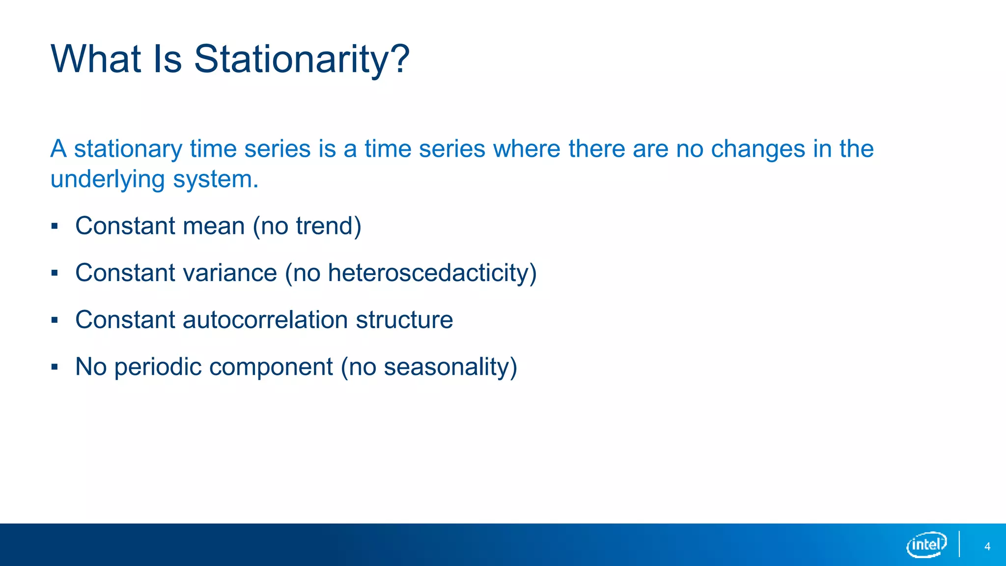
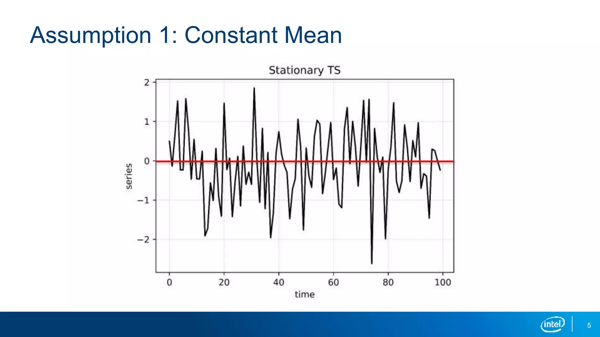
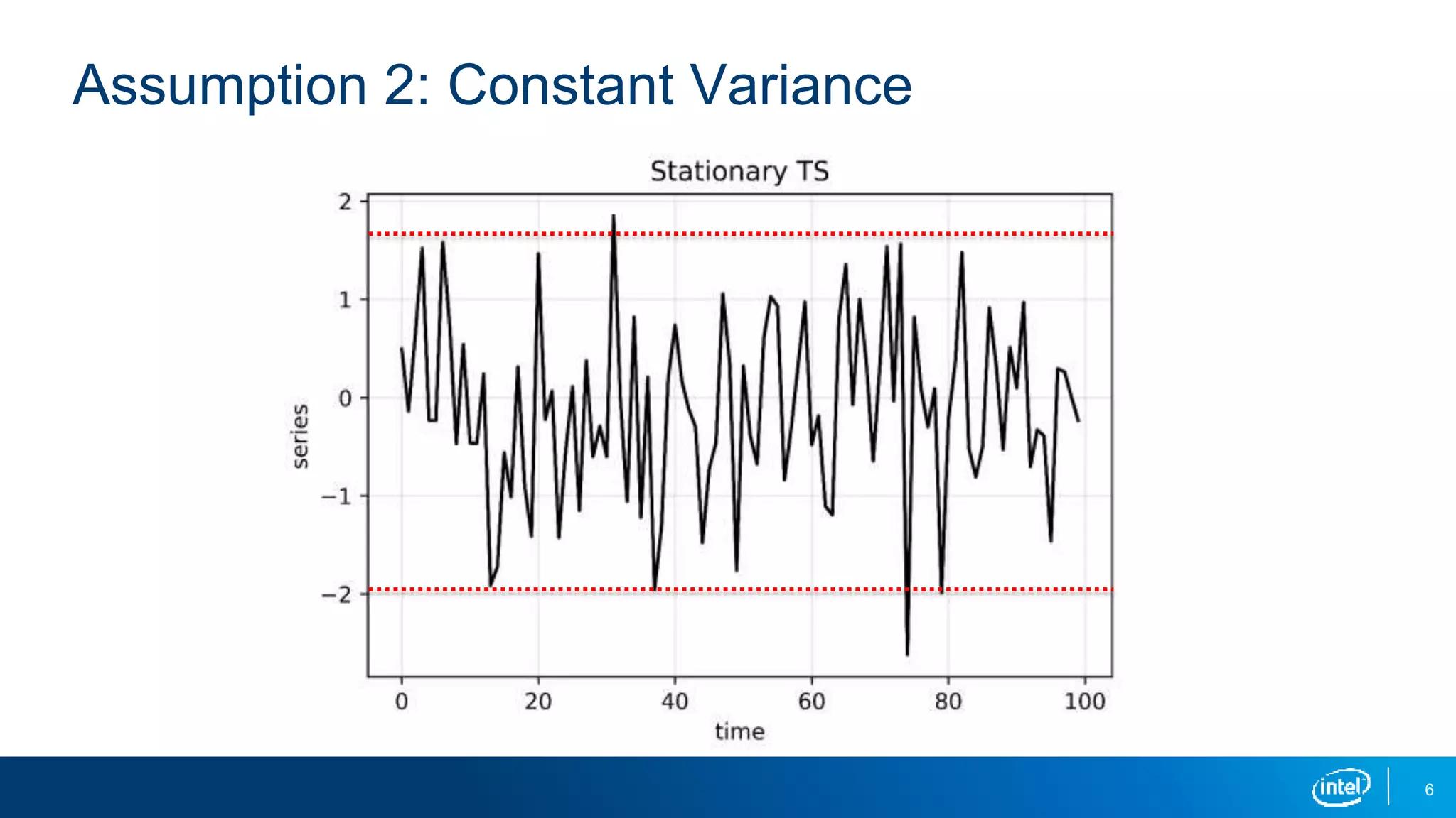
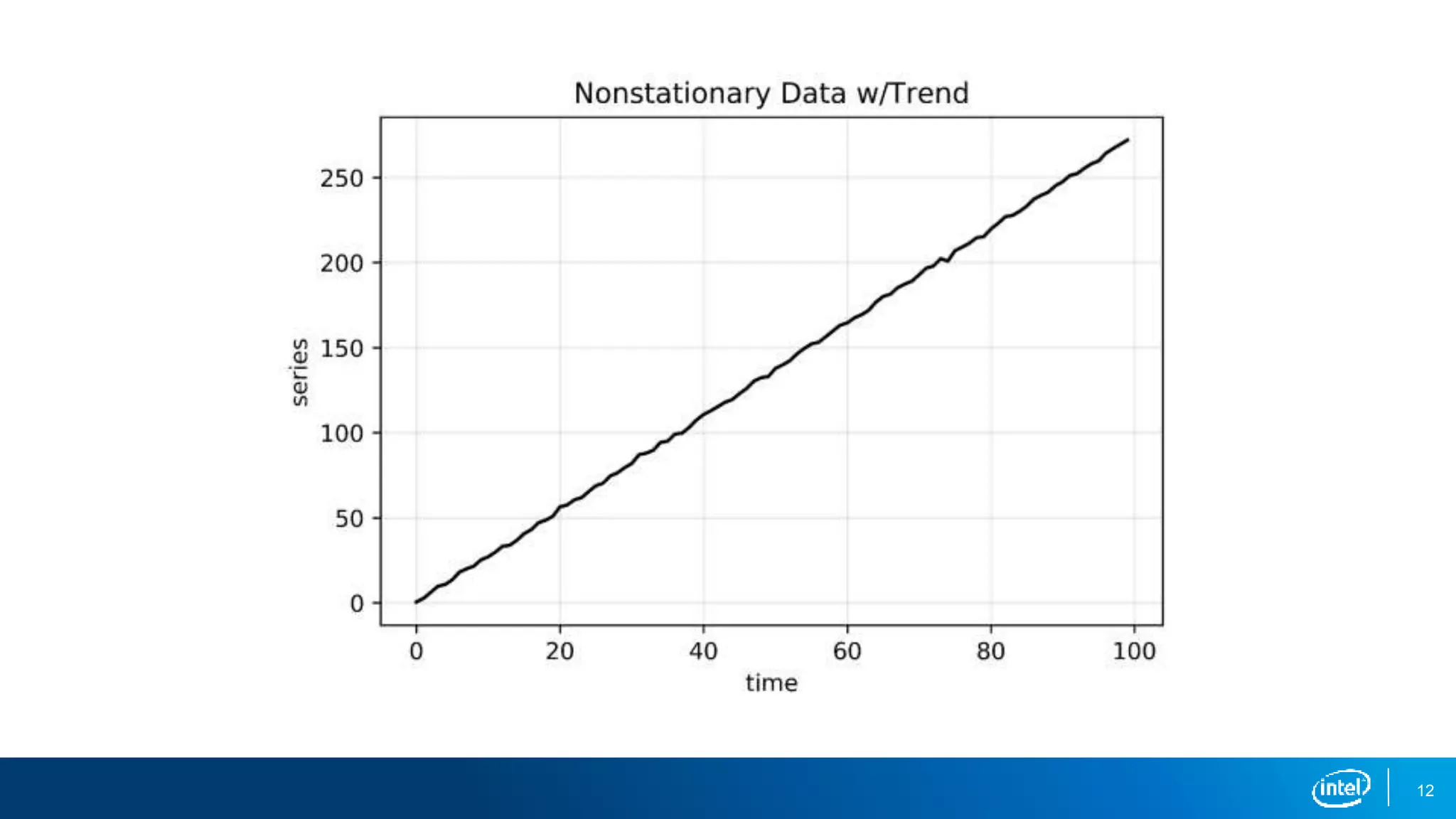
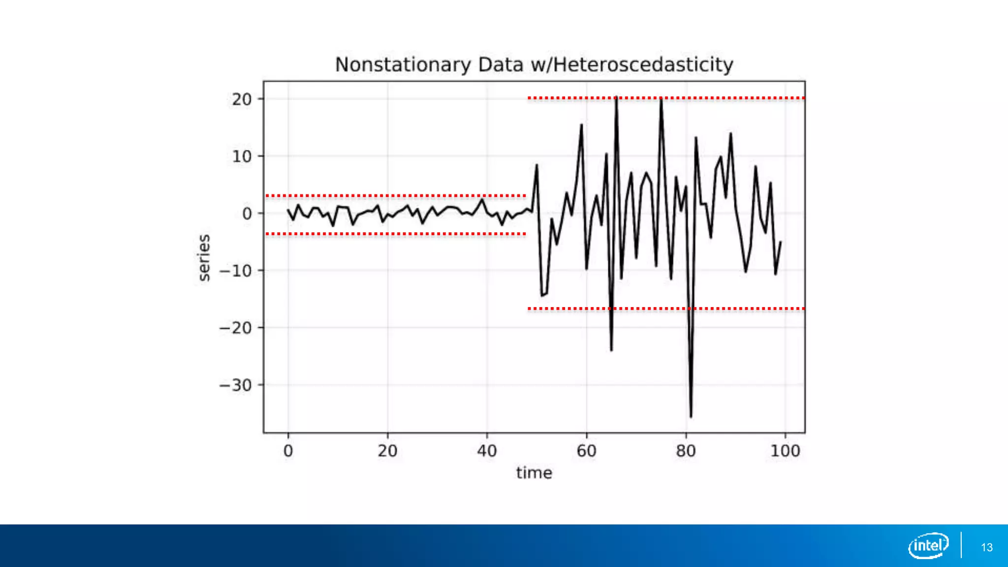
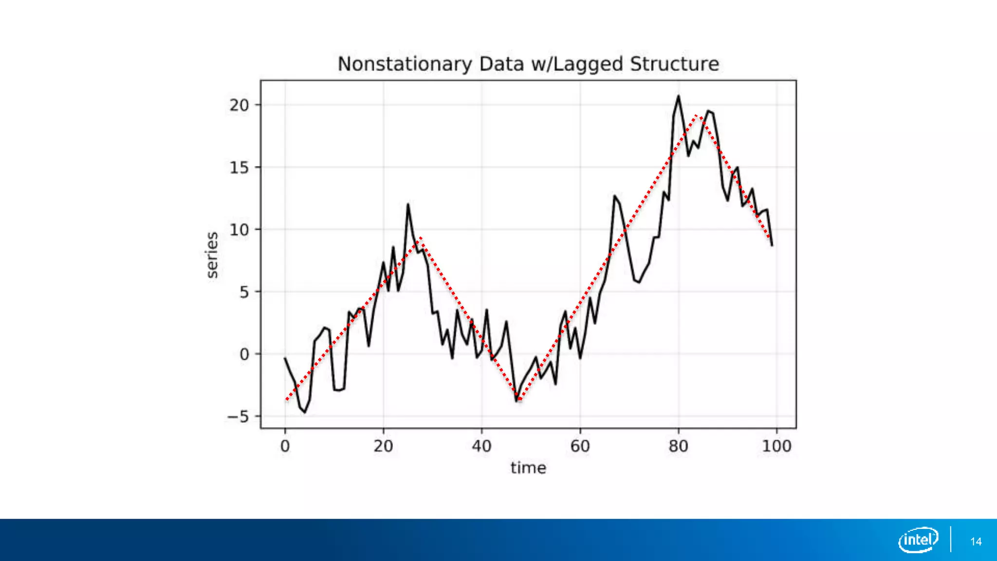
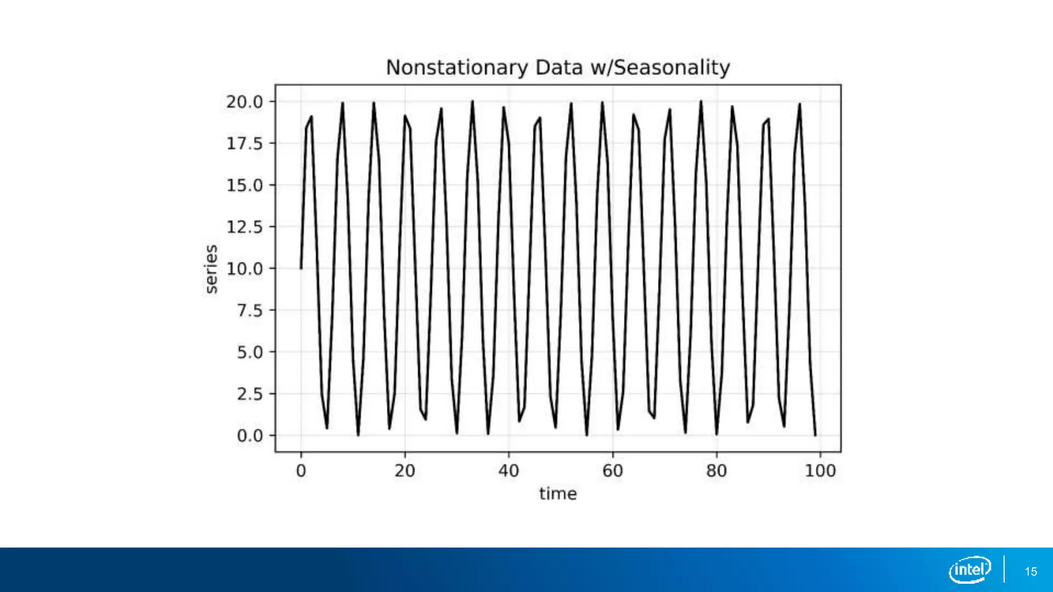
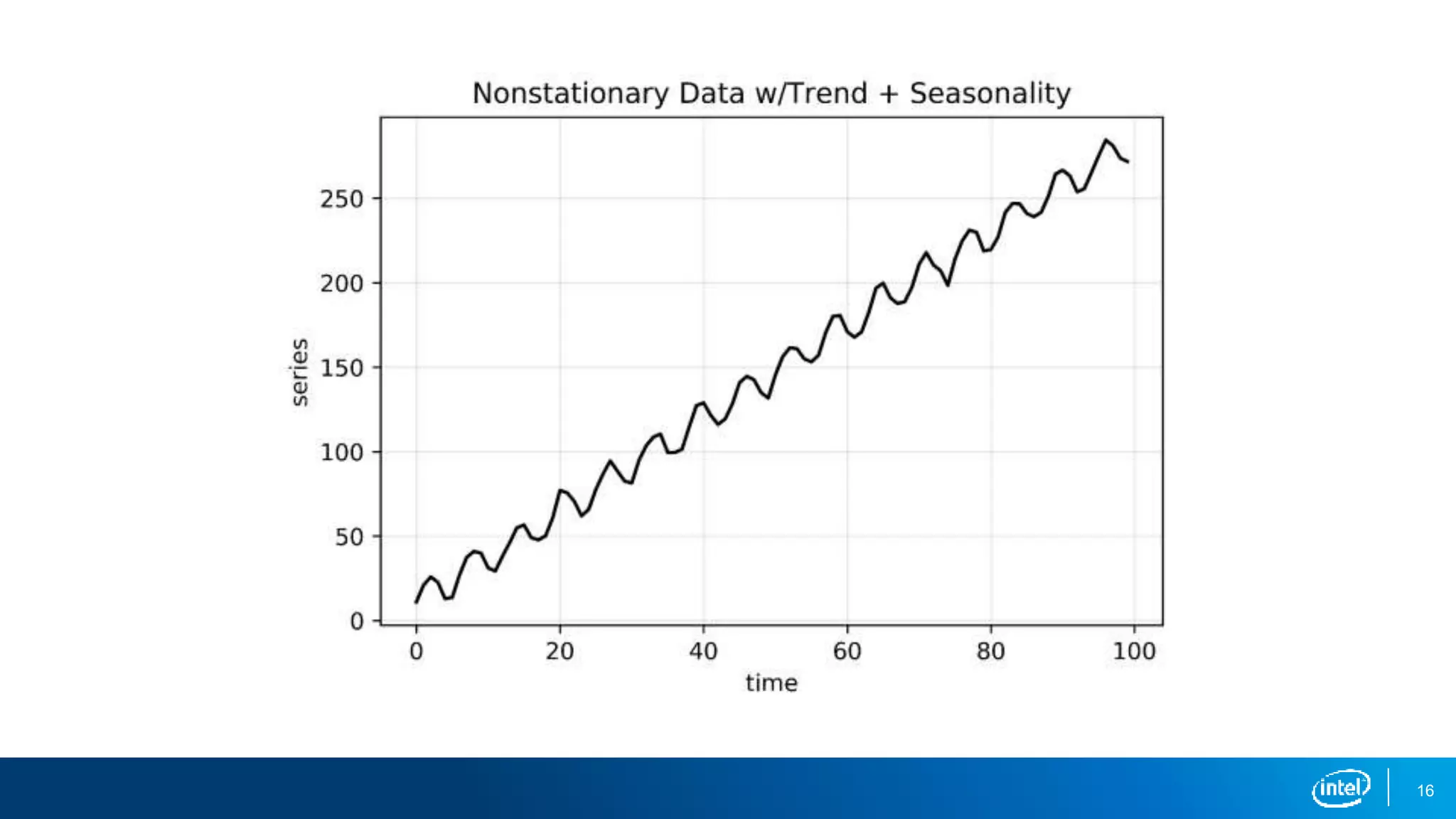
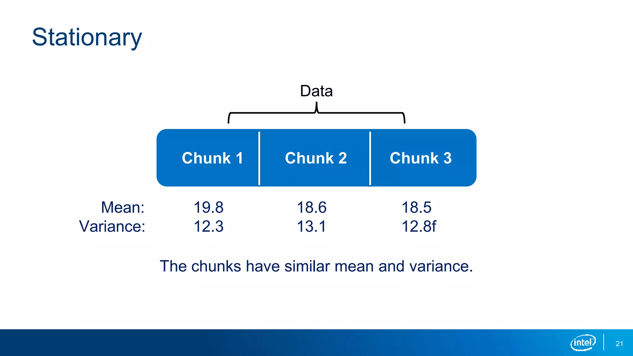
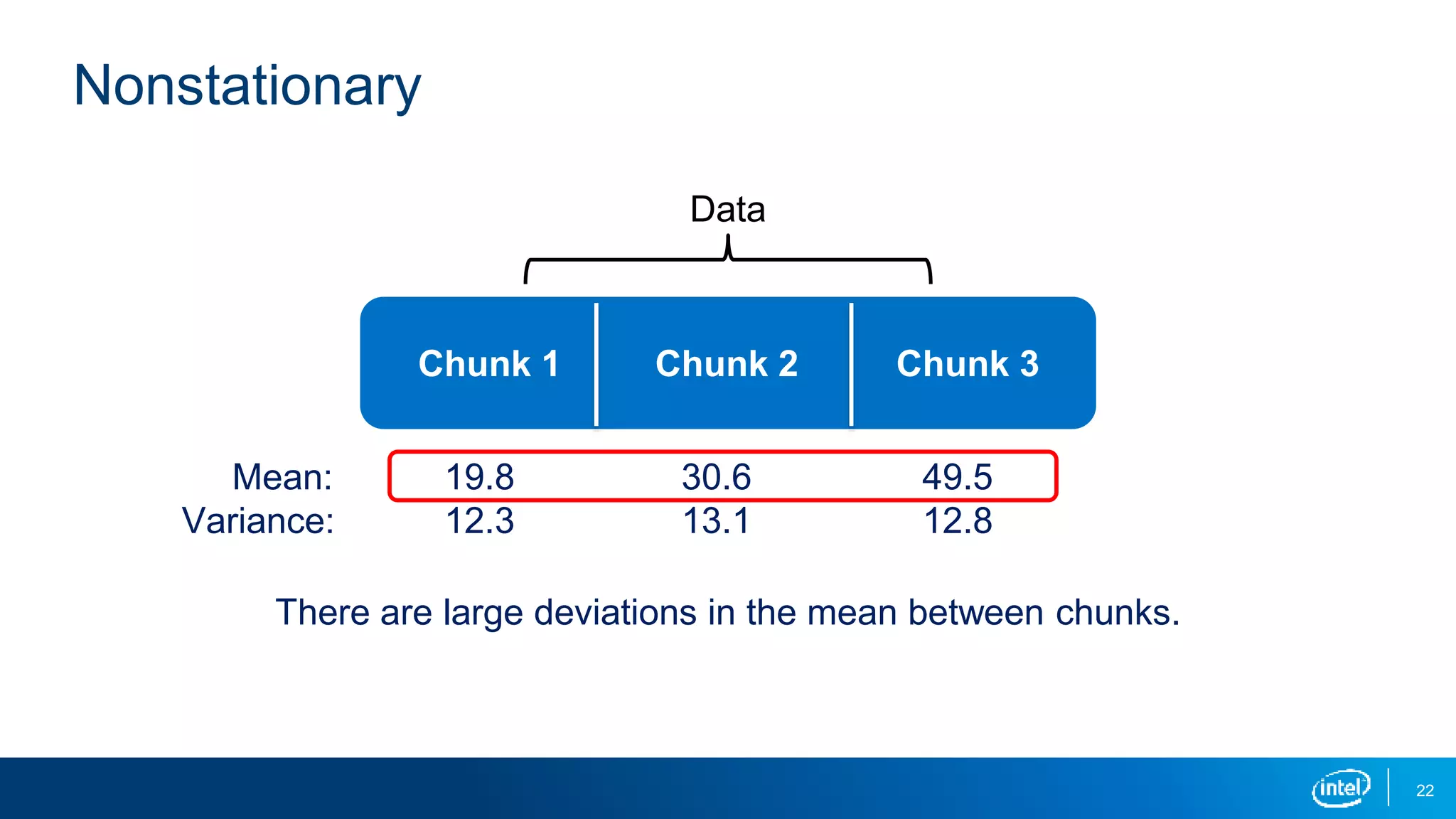
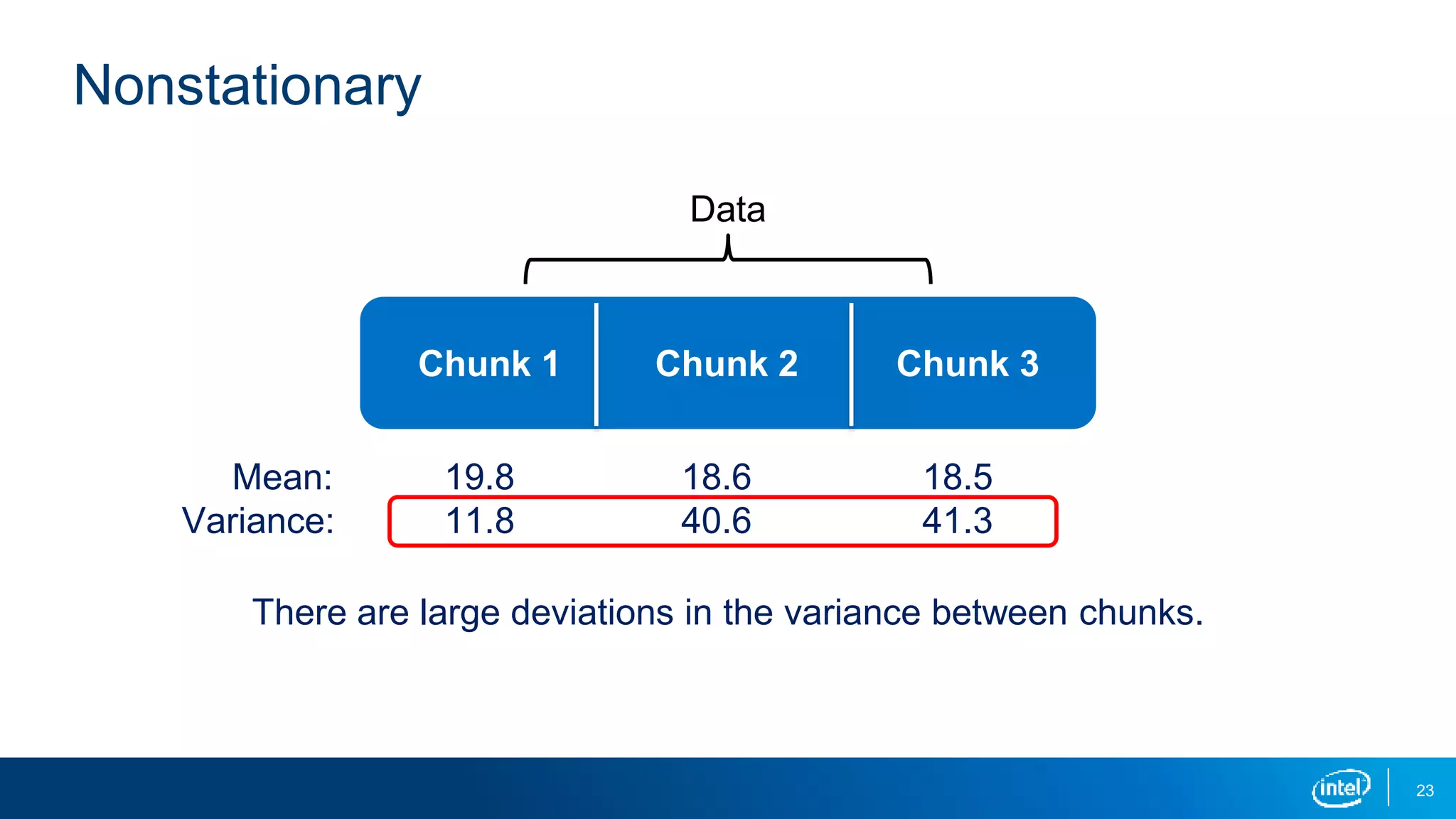
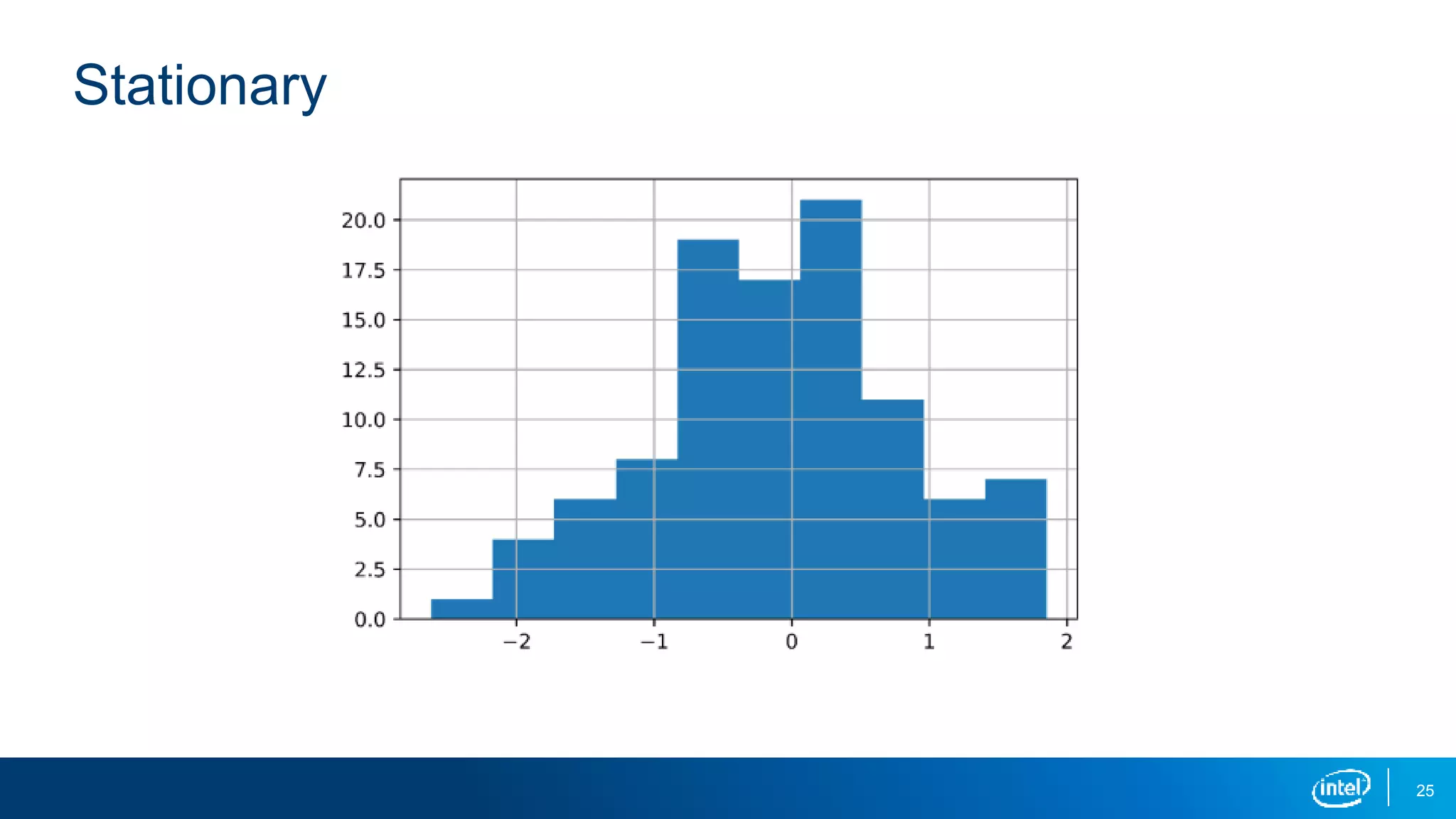
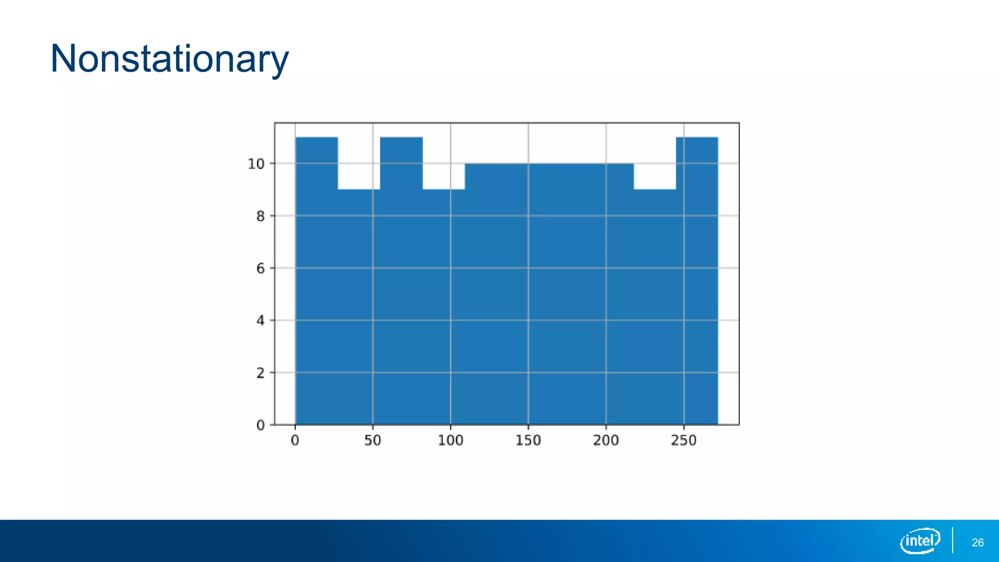
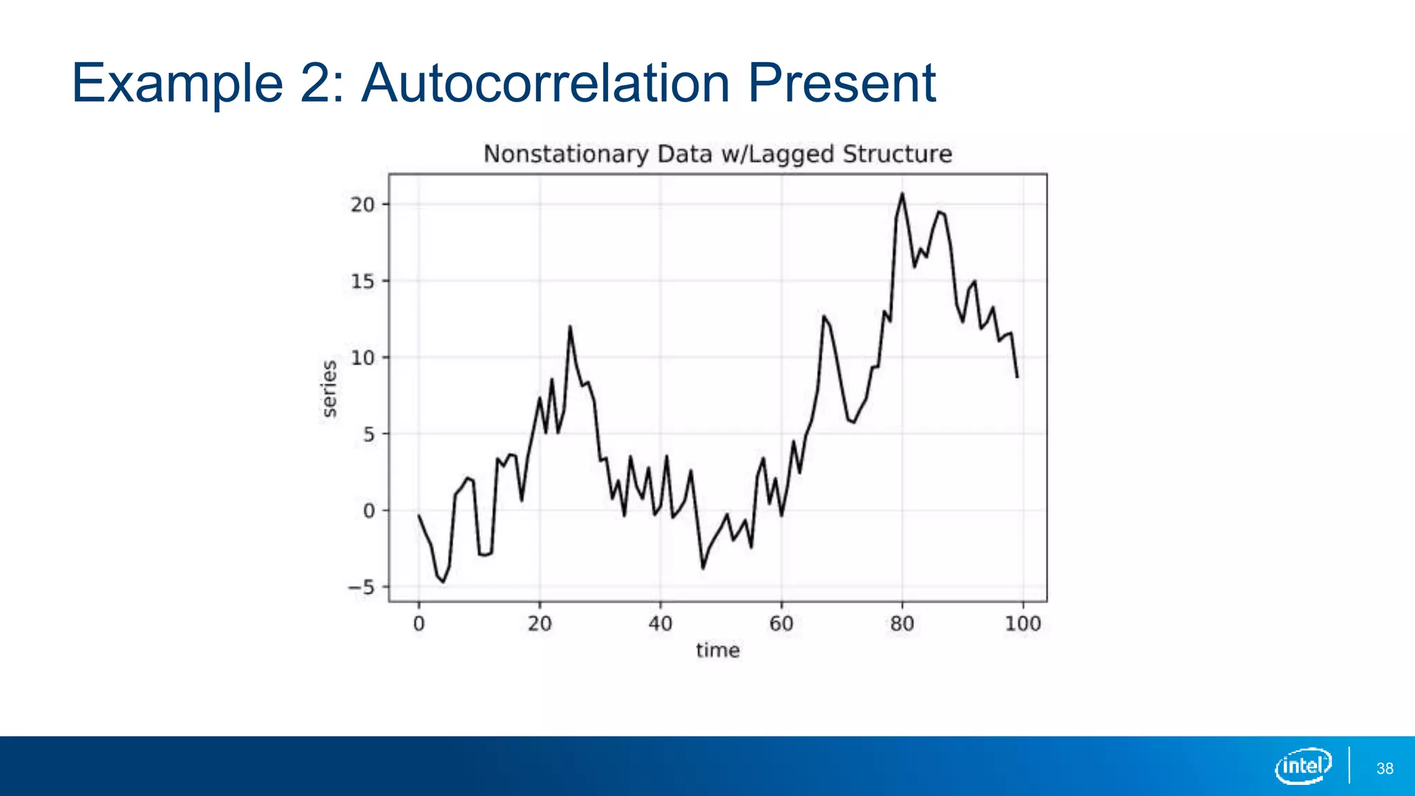
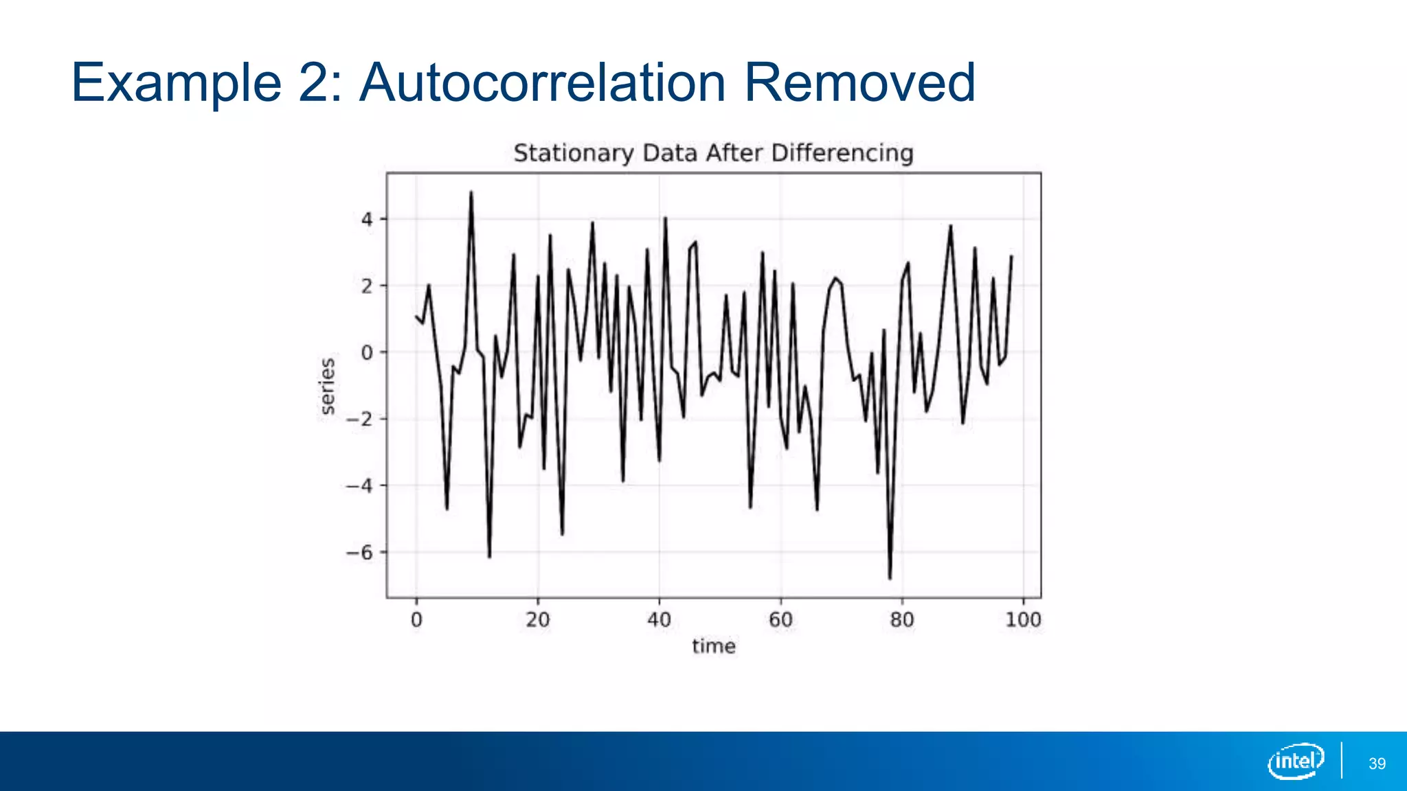
1. Lesson 2: Stationary Time Series

2. 2
Learning Objectives
You will be able to do the following:
▪ Define "stationarity."
▪ Describe methods for determining stationarity.
▪ Explain how to transform nonstationary time-series data.
▪ Use Python* to identify and transform nonstationary time-series data.

4. 4
What Is Stationarity?
A stationary time series is a time series where there are no changes in the
underlying system.
▪ Constant mean (no trend)
▪ Constant variance (no heteroscedacticity)
▪ Constant autocorrelation structure
▪ No periodic component (no seasonality)

5. 5
Assumption 1: Constant Mean

6. 6
Assumption 2: Constant Variance

7. 7
Autocorrelation
Autocorrelation is a key concept in time-series analysis.
▪ Autocorrelation is the correlation between a measurement at two
different times.
▪ The time interval between values is called the lag.
▪ For example, stock prices may be correlated from one day to the next
with a lag value of 1.
▪ Autocorrelation often results in a pattern, whereas a time series without
autocorrelation will exhibit randomness.

8. 8
No autocorrelation Has autocorrelation

9. 9
Assumption 3: Constant Autocorrelation Structure
A stationary time series has constant autocorrelation structure throughout
the entire series.
▪ If the autocorrelation remains constant throughout the series, a simple
transformation can be used to remove the autocorrelation.
▪ This will be useful for several future models.

10. 10
Why Is Stationarity Important?
Stationarity is a fundamental assumption in many time-series forecasting
models:
▪ Without it many basic time-series models would break down.
▪ Transformations can be applied to convert a nonstationary time series to a
stationary one before modeling.
▪ While there are more advanced time-series models that can handle
nonstationary data, that is beyond the scope of this lesson.

12. 12

13. 13

14. 14

15. 15

16. 16

18. 18
How to Identify Nonstationary Time-Series Data
There are several ways to identify nonstationary time-series data:
▪ Run-sequence plots
▪ Summary statistics
▪ Histogram plot
▪ Augmented Dickey-Fuller test

19. 19
Run-Sequence Plot
A run-sequence plot is simply a plot of your time-series data.
▪ This should always be your first step in time-series analysis.
▪ It often shows whether there is underlying structure.
▪ Be on the lookout for trend, seasonality, and autocorrelation.
▪ The previous plots are great examples.

20. 20
Summary Statistics
Calculating the mean and variance over time is a useful way to discern
whether the series is stationary.
▪ A simple but effective way to do this is to split your data into chunks over
time and compute statistics for each chunk.
▪ Large deviations in either the mean or the variance among chunks are
problematic and mean that your data is nonstationary.

21. 21
Stationary
Data
Chunk 1 Chunk 2 Chunk 3
Mean:
Variance:
The chunks have similar mean and variance.
19.8
12.3
18.6
13.1
18.5
12.8f

22. 22
Nonstationary
Data
Chunk 1 Chunk 2 Chunk 3
Mean:
Variance:
19.8
12.3
30.6
13.1
49.5
12.8
There are large deviations in the mean between chunks.

23. 23
Nonstationary
Data
Chunk 1 Chunk 2 Chunk 3
Mean:
Variance:
There are large deviations in the variance between chunks.
19.8
11.8
18.6
40.6
18.5
41.3

24. 24
Histogram Plot
A histogram plot gives important clues into a time series’ underlying structure.
▪ If you see a distribution that is approximately normal, that’s a good indication
your time series is stationary.
▪ If you see a nonnormal distribution, that’s a good indication your time series is
nonstationary.

25. 25
Stationary

26. 26
Nonstationary

27. 27
Augmented Dickey-Fuller Test
The Augmented Dickey-Fuller test is a hypothesis test that tests specifically
for stationarity.
▪ We generally say that the series is nonstationary if the p-value is less than
0.05.
▪ It is a less appropriate test to use with small datasets or when
heteroscedasticity is present.
▪ It is best to pair ADF with other techniques, such as run-sequence plots,
summary statistics, or histograms.

29. 29
How to Transform Nonstationary Time-Series Data
There are several ways to transform nonstationary time-series data:
▪ Remove trend (constant mean)
▪ Remove heteroscedasticity with log (constant variance)
▪ Remove autocorrelation with differencing (exploit constant structure)
▪ Remove seasonality (no periodic component)
▪ Oftentimes you’ll have to do several of these on one dataset!

30. 30
Example 1: Trend & Seasonality Present
A time series with a trend or seasonality component is a nonstationary series. To
make it stationary, we can do the following:
▪ Subtract the trend so that the series has constant mean.
▪ Subtract the seasonality so that the series has no periodic component.

31. 31
Example 1: Trend & Seasonality Components

32. 32
Example 1: Trend & Seasonality Components

33. 33
Example 1: Trend & Seasonality Removed

34. 34
Example 2: Heteroscedasticity Present
A time series with differing variances in two distinct regions is a nonstationary
series. To make it stationary, we can do the following:
▪ Apply the log transformation.
▪ This squashes the larger values so that the variances are closer.

35. 35
Example 2: Heteroscedasticity Present

36. 36
Example 2: Heteroscedasticity Squashed

37. 37
Example 3: Autocorrelation Present
Say a given time series has autocorrelation with a lag of 1. By definition, this is
a nonstationary series in its current form. To make it stationary, we can do the
following:
▪ Difference the data by subtracting by a specific lag.
▪ How you determine the appropriate lag will be covered in the future during
Lesson 4.

38. 38
Example 2: Autocorrelation Present

39. 39
Example 2: Autocorrelation Removed

41. 41
Use Python to Identify and Transform Nonstationarity
Next up is a look at applying these concepts in Python.
▪ See notebook entitled Introduction_to_Stationarity_student.ipynb

42. 42
Learning Objectives Recap
In this session you learned how to do the following:
▪ Define "stationarity"
▪ Describe methods for determining stationarity
▪ Explain how to transform nonstationary time-series data
▪ Use Python to identify and transform nonstationary time-series data

43. Legal Notices and Disclaimers
This presentation is for informational purposes only. INTEL MAKES NO WARRANTIES, EXPRESS OR IMPLIED, IN THIS
SUMMARY.
Intel technologies’ features and benefits depend on system configuration and may require enabled hardware, software or
service activation. Performance varies depending on system configuration. Check with your system manufacturer or
retailer or learn more at intel.com.
Sample source code is released under the Intel Sample Source Code License Agreement.
Intel, the Intel logo, the Intel. Experience What’s Inside logo, and Intel. Experience What’s Inside are trademarks of Intel
Corporation in the U.S. and/or other countries.
*Other names and brands may be claimed as the property of others.
Copyright © 2018, Intel Corporation. All rights reserved.
43