Introduction - Objectives Of Studying Time Series Analysis - Variations In Time Series
- Methods Of Estimating Trend: Freehand Method - Moving Average Method - Semi-Average Method - Least
Square Method
Introduction - Objectives Of Studying Time Series Analysis - Variations In Time Series
- Methods Of Estimating Trend: Freehand Method - Moving Average Method - Semi-Average Method - Least
Square Method
Chapter 6 part1- Introduction to Inference-Estimating with Confidence (Introd...nszakir
Introduction to Inference, Estimating with Confidence, Inference, Statistical Confidence, Confidence Intervals, Confidence Interval for a Population Mean, Choosing the Sample Size
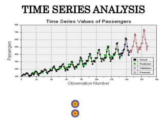
1) To understand the underlying structure of Time Series represented by sequence of observations by breaking it down to its components.
2) To fit a mathematical model and proceed to forecast the future.
Introduction to Statistics - Basic concepts
- How to be a good doctor - A step in Health promotion
- By Ibrahim A. Abdelhaleem - Zagazig Medical Research Society (ZMRS)
Time Series basic concepts and ARIMA family of models. There is an associated video session along with code in github: https://github.com/bhaskatripathi/timeseries-autoregressive-models
https://drive.google.com/file/d/1yXffXQlL6i4ufQLSpFFrJgymhHNXL1Mf/view?usp=sharing
Chapter 6 part1- Introduction to Inference-Estimating with Confidence (Introd...nszakir
Introduction to Inference, Estimating with Confidence, Inference, Statistical Confidence, Confidence Intervals, Confidence Interval for a Population Mean, Choosing the Sample Size
1) To understand the underlying structure of Time Series represented by sequence of observations by breaking it down to its components.
2) To fit a mathematical model and proceed to forecast the future.
Introduction to Statistics - Basic concepts
- How to be a good doctor - A step in Health promotion
- By Ibrahim A. Abdelhaleem - Zagazig Medical Research Society (ZMRS)
Time Series basic concepts and ARIMA family of models. There is an associated video session along with code in github: https://github.com/bhaskatripathi/timeseries-autoregressive-models
https://drive.google.com/file/d/1yXffXQlL6i4ufQLSpFFrJgymhHNXL1Mf/view?usp=sharing
Moving avg & method of least squareHassan Jalil
A quantitative method of forecasting or smoothing a time series by averaging each successive group (no. of observations) of data values.
Term MOVING is used because it is obtained by summing and averaging the values from a given no of periods, each time deleting the oldest value and adding a new value.
Basic Concepts, Components of time series. The trend, Fitting of trend by least square method and moving average method, uses of time series in business.
Statistics assignment and homework help serviceTutor Help Desk
Looking for quality statistics assignment and homework help? Tutorhelpdesk offers you complete range of expert academic help for all grades of statistics projects at most realistic cost. We honor your timeline and are reachable 24x7 online at your service.
A Numerical Case Study on the subject Business Statistics and the use of Time Series Analysis as a tool to solve various problems related to business decisions.
Stuck with your Forecasting Assignment? Get 24/7 help from tutors with Phd in the subject. Email us at support@helpwithassignment.com
Reach us at http://www.HelpWithAssignment.com
Welcome to TechSoup New Member Orientation and Q&A (May 2024).pdfTechSoup
In this webinar you will learn how your organization can access TechSoup's wide variety of product discount and donation programs. From hardware to software, we'll give you a tour of the tools available to help your nonprofit with productivity, collaboration, financial management, donor tracking, security, and more.
2024.06.01 Introducing a competency framework for languag learning materials ...Sandy Millin
http://sandymillin.wordpress.com/iateflwebinar2024
Published classroom materials form the basis of syllabuses, drive teacher professional development, and have a potentially huge influence on learners, teachers and education systems. All teachers also create their own materials, whether a few sentences on a blackboard, a highly-structured fully-realised online course, or anything in between. Despite this, the knowledge and skills needed to create effective language learning materials are rarely part of teacher training, and are mostly learnt by trial and error.
Knowledge and skills frameworks, generally called competency frameworks, for ELT teachers, trainers and managers have existed for a few years now. However, until I created one for my MA dissertation, there wasn’t one drawing together what we need to know and do to be able to effectively produce language learning materials.
This webinar will introduce you to my framework, highlighting the key competencies I identified from my research. It will also show how anybody involved in language teaching (any language, not just English!), teacher training, managing schools or developing language learning materials can benefit from using the framework.
Instructions for Submissions thorugh G- Classroom.pptxJheel Barad
This presentation provides a briefing on how to upload submissions and documents in Google Classroom. It was prepared as part of an orientation for new Sainik School in-service teacher trainees. As a training officer, my goal is to ensure that you are comfortable and proficient with this essential tool for managing assignments and fostering student engagement.
Honest Reviews of Tim Han LMA Course Program.pptxtimhan337
Personal development courses are widely available today, with each one promising life-changing outcomes. Tim Han’s Life Mastery Achievers (LMA) Course has drawn a lot of interest. In addition to offering my frank assessment of Success Insider’s LMA Course, this piece examines the course’s effects via a variety of Tim Han LMA course reviews and Success Insider comments.
Operation “Blue Star” is the only event in the history of Independent India where the state went into war with its own people. Even after about 40 years it is not clear if it was culmination of states anger over people of the region, a political game of power or start of dictatorial chapter in the democratic setup.
The people of Punjab felt alienated from main stream due to denial of their just demands during a long democratic struggle since independence. As it happen all over the word, it led to militant struggle with great loss of lives of military, police and civilian personnel. Killing of Indira Gandhi and massacre of innocent Sikhs in Delhi and other India cities was also associated with this movement.
The French Revolution, which began in 1789, was a period of radical social and political upheaval in France. It marked the decline of absolute monarchies, the rise of secular and democratic republics, and the eventual rise of Napoleon Bonaparte. This revolutionary period is crucial in understanding the transition from feudalism to modernity in Europe.
For more information, visit-www.vavaclasses.com
A Strategic Approach: GenAI in EducationPeter Windle
Artificial Intelligence (AI) technologies such as Generative AI, Image Generators and Large Language Models have had a dramatic impact on teaching, learning and assessment over the past 18 months. The most immediate threat AI posed was to Academic Integrity with Higher Education Institutes (HEIs) focusing their efforts on combating the use of GenAI in assessment. Guidelines were developed for staff and students, policies put in place too. Innovative educators have forged paths in the use of Generative AI for teaching, learning and assessments leading to pockets of transformation springing up across HEIs, often with little or no top-down guidance, support or direction.
This Gasta posits a strategic approach to integrating AI into HEIs to prepare staff, students and the curriculum for an evolving world and workplace. We will highlight the advantages of working with these technologies beyond the realm of teaching, learning and assessment by considering prompt engineering skills, industry impact, curriculum changes, and the need for staff upskilling. In contrast, not engaging strategically with Generative AI poses risks, including falling behind peers, missed opportunities and failing to ensure our graduates remain employable. The rapid evolution of AI technologies necessitates a proactive and strategic approach if we are to remain relevant.
Synthetic Fiber Construction in lab .pptxPavel ( NSTU)
Synthetic fiber production is a fascinating and complex field that blends chemistry, engineering, and environmental science. By understanding these aspects, students can gain a comprehensive view of synthetic fiber production, its impact on society and the environment, and the potential for future innovations. Synthetic fibers play a crucial role in modern society, impacting various aspects of daily life, industry, and the environment. ynthetic fibers are integral to modern life, offering a range of benefits from cost-effectiveness and versatility to innovative applications and performance characteristics. While they pose environmental challenges, ongoing research and development aim to create more sustainable and eco-friendly alternatives. Understanding the importance of synthetic fibers helps in appreciating their role in the economy, industry, and daily life, while also emphasizing the need for sustainable practices and innovation.
The Roman Empire A Historical Colossus.pdfkaushalkr1407
The Roman Empire, a vast and enduring power, stands as one of history's most remarkable civilizations, leaving an indelible imprint on the world. It emerged from the Roman Republic, transitioning into an imperial powerhouse under the leadership of Augustus Caesar in 27 BCE. This transformation marked the beginning of an era defined by unprecedented territorial expansion, architectural marvels, and profound cultural influence.
The empire's roots lie in the city of Rome, founded, according to legend, by Romulus in 753 BCE. Over centuries, Rome evolved from a small settlement to a formidable republic, characterized by a complex political system with elected officials and checks on power. However, internal strife, class conflicts, and military ambitions paved the way for the end of the Republic. Julius Caesar’s dictatorship and subsequent assassination in 44 BCE created a power vacuum, leading to a civil war. Octavian, later Augustus, emerged victorious, heralding the Roman Empire’s birth.
Under Augustus, the empire experienced the Pax Romana, a 200-year period of relative peace and stability. Augustus reformed the military, established efficient administrative systems, and initiated grand construction projects. The empire's borders expanded, encompassing territories from Britain to Egypt and from Spain to the Euphrates. Roman legions, renowned for their discipline and engineering prowess, secured and maintained these vast territories, building roads, fortifications, and cities that facilitated control and integration.
The Roman Empire’s society was hierarchical, with a rigid class system. At the top were the patricians, wealthy elites who held significant political power. Below them were the plebeians, free citizens with limited political influence, and the vast numbers of slaves who formed the backbone of the economy. The family unit was central, governed by the paterfamilias, the male head who held absolute authority.
Culturally, the Romans were eclectic, absorbing and adapting elements from the civilizations they encountered, particularly the Greeks. Roman art, literature, and philosophy reflected this synthesis, creating a rich cultural tapestry. Latin, the Roman language, became the lingua franca of the Western world, influencing numerous modern languages.
Roman architecture and engineering achievements were monumental. They perfected the arch, vault, and dome, constructing enduring structures like the Colosseum, Pantheon, and aqueducts. These engineering marvels not only showcased Roman ingenuity but also served practical purposes, from public entertainment to water supply.
Acetabularia Information For Class 9 .docxvaibhavrinwa19
Acetabularia acetabulum is a single-celled green alga that in its vegetative state is morphologically differentiated into a basal rhizoid and an axially elongated stalk, which bears whorls of branching hairs. The single diploid nucleus resides in the rhizoid.
Embracing GenAI - A Strategic ImperativePeter Windle
Artificial Intelligence (AI) technologies such as Generative AI, Image Generators and Large Language Models have had a dramatic impact on teaching, learning and assessment over the past 18 months. The most immediate threat AI posed was to Academic Integrity with Higher Education Institutes (HEIs) focusing their efforts on combating the use of GenAI in assessment. Guidelines were developed for staff and students, policies put in place too. Innovative educators have forged paths in the use of Generative AI for teaching, learning and assessments leading to pockets of transformation springing up across HEIs, often with little or no top-down guidance, support or direction.
This Gasta posits a strategic approach to integrating AI into HEIs to prepare staff, students and the curriculum for an evolving world and workplace. We will highlight the advantages of working with these technologies beyond the realm of teaching, learning and assessment by considering prompt engineering skills, industry impact, curriculum changes, and the need for staff upskilling. In contrast, not engaging strategically with Generative AI poses risks, including falling behind peers, missed opportunities and failing to ensure our graduates remain employable. The rapid evolution of AI technologies necessitates a proactive and strategic approach if we are to remain relevant.
2. Definition:
“A time series is a set of observation taken at specified times,
usually at equal intervals”.
“A time series may be defined as a collection of reading belonging to
different time periods of some economic or composite variables”.
By –Ya-Lun-Chau
Time series establish relation between “cause” & “Effects”.
One variable is “Time” which is independent variable & and the
second is “Data” which is the dependent variable.
3. We explain it from the following example:
• From example 1 it is clear that the sale of milk packets is decrease
from Monday to Friday then again its start to increase.
• Same thing in example 2 the population is continuously increase.
Day No. of Packets of milk sold
Monday 90
Tuesday 88
Wednesday 85
Thursday 75
Friday 72
Saturday 90
Sunday 102
Year Population (in Million)
1921 251
1931 279
1941 319
1951 361
1961 439
1971 548
1981 685
4. Importance of Time Series Analysis:-
As the basis of Time series Analysis businessman can
predict about the changes in economy. There are
following points which clear about the its importance:
1. Profit of experience.
2. Safety from future
3. Utility Studies
4. Sales Forecasting 5. Budgetary Analysis
6. Stock Market Analysis 7. Yield Projections
8. Process and Quality Control
9. Inventory Studies
10. Economic Forecasting
11. Risk Analysis & Evaluation of changes.
12. Census Analysis
5. Components of Time Series:-
The change which are effected by Economic, Social,
Natural, Industrial & Political Reasons. These reasons
are called components of Time Series.
Secular trend :-
Seasonal variation :-
Cyclical variation :-
Irregular variation :-
12. Random or Irregular
Component
• Erratic, Nonsystematic, Random, ‘Residual’
Fluctuations
• Due to Random Variations of
– Nature
– Accidents
– Flood
– War
• Short Duration and Non-repeating
13. Time Series Model
• Addition Model:
Y = T + S + C + I
Where:- Y = value of the variable at time t
T = Trend Value
S = Seasonal Fluctuation
C = Cyclical Fluctuation
I = Irregular variation
I =
I = Irregular
Fluctuation
• Multiplication Model:
Y = T x S x C x I
or
Y = TSCI
14. Measurement of Trend:-
• The following methods are used for calculation
of trend:
Free Hand Curve Method:
Semi – Average Method:
Moving Average Method:
Least Square Method:
15. Free hand Curve Method:-
• In this method the data is denoted on graph paper. We
take “Time” on ‘x’ axis and “Data” on the ‘y’ axis. On
graph there will be a point for every point of time. We
make a smooth hand curve with the help of this plotted
points.
Example:
Draw a free hand curve on the basis of the
following data:
Years 1989 1990 1991 1992 1993 1994 1995 1996
Profit
(in
‘000)
148 149 149.5 149 150.5 152.2 153.7 153
17. Semi – Average Method:-
• In this method the given data are divided in two parts,
preferable with the equal number of years.
• For example, if we are given data from 1991 to 2008,
i.e., over a period of 18 years, the two equal parts will be
first nine years, i.e.,1991 to 1999 and from 2000 to
2008. In case of odd number of years like, 9, 13, 17, etc..,
two equal parts can be made simply by ignoring the
middle year. For example, if data are given for 19 years
from 1990 to 2007 the two equal parts would be from
1990 to 1998 and from 2000 to 2008 - the middle year
1999 will be ignored.
18. • Example:
Find the trend line from the
following data by Semi – Average Method:-
Year 1989 1990 1991 1992 1993 1994 1995 1996
Production
(M.Ton.)
150 152 153 151 154 153 156 158
There are total 8 trends. Now we distributed it in equal part.
Now we calculated Average mean for every part.
First Part = 150 + 152 + 153 + 151 = 151.50
4
Second Part = 154 + 153 + 156 + 158 = 155.25
4
21. Moving Average Method:-
• It is one of the most popular method for calculating Long Term
Trend. This method is also used for ‘Seasonal fluctuation’, ‘cyclical
fluctuation’ & ‘irregular fluctuation’. In this method we calculate
the ‘Moving Average for certain years.
• For example: If we calculating ‘Three year’s Moving Average’ then
according to this method:
=(1)+(2)+(3) , (2)+(3)+(4) , (3)+(4)+(5), ……………..
3 3 3
Where (1),(2),(3),………. are the various years of time series.
Example: Find out the five year’s moving Average:
Year 1982 1983 1984 1985 1986 1987 1988 1989 1990 1991 1992 1993 1994 1995 1996
Price 20 25 33 33 27 35 40 43 35 32 37 48 50 37 45
23. • This method is most widely in practice. When this method is
applied, a trend line is fitted to data in such a manner that
the following two conditions are satisfied:-
The sum of deviations of the actual values of y and computed
values of y is zero.
i.e., the sum of the squares of the deviation of the actual and
computed values is least from this line. That is why method is
called the method of least squares. The line obtained by this
method is known as the line of `best fit`.
is least
Least Square Method:-
0
c
Y
Y
2
c
Y
Y
24. The Method of least square can be used either to fit a straight line
trend or a parabolic trend.
The straight line trend is represented by the equation:-
= Yc = a + bx
Where, Y = Trend value to be computed
X = Unit of time (Independent Variable)
a = Constant to be Calculated
b = Constant to be calculated
Example:-
Draw a straight line trend and estimate trend value for 1996:
Year 1991 1992 1993 1994 1995
Production 8 9 8 9 16
25. Year
(1)
Deviation From
1990
X
(2)
Y
(3)
XY
(4)
X2
(5)
Trend
Yc = a + bx
(6)
1991
1992
1993
1994
1995
1
2
3
4
5
8
9
8
9
16
8
18
24
36
80
1
4
9
16
25
5.2 + 1.6(1) = 6.8
5.2 + 1.6(2) = 8.4
5.2 + 1.6(3) = 10.0
5.2 + 1.6(4) = 11.6
5.2 + 1.6(5) = 13.2
N= 5
= 15 =50 = 166 = 55
X
Y XY 2
X
’
Now we calculate the value of two constant ‘a’ and ‘b’ with the help
of two equation:-
Solution:-
26.
2
X
b
X
a
XY
X
b
Na
Y
Now we put the value of :-
50 = 5a + 15(b) ……………. (i)
166 = 15a + 55(b) ……………… (ii)
Or 5a + 15b = 50 ……………… (iii)
15a + 55b = 166 …………………. (iv)
Equation (iii) Multiply by 3 and subtracted by (iv)
-10b = -16
b = 1.6
Now we put the value of “b” in the equation (iii)
N
X
XY
Y
X ,&
,
,
, 2
27. = 5a + 15(1.6) = 50
5a = 26
a = = 5.2
As according the value of ‘a’ and ‘b’ the trend line:-
Yc = a + bx
Y= 5.2 + 1.6X
Now we calculate the trend line for 1996:-
Y1996 = 5.2 + 1.6 (6) = 14.8
5
26
28. Shifting The Trend Origin:-
• In above Example the trend equation is:
Y = 5.2 + 1.6x
Here the base year is 1993 that means actual base of these
year will 1st July 1993. Now we change the base year in
1991. Now the base year is back 2 years unit than
previous base year.
Now we will reduce the twice of the value of the ‘b’
from the value of ‘a’.
Then the new value of ‘a’ = 5.2 – 2(1.6)
Now the trend equation on the basis of year 1991:
Y = 2.0+ 1.6x
29. Parabolic Curve:-
Many times the line which draw by “Least Square Method”
is not prove ‘Line of best fit’ because it is not present
actual long term trend So we distributed Time Series in sub-
part and make following equation:-
Yc = a + bx + cx2
If this equation is increase up to second degree then it is “Parabola
of second degree” and if it is increase up to third degree then it
“Parabola of third degree”. There are three constant ‘a’, ‘b’ and ‘c’.
Its are calculated by following three equation:-
30. If we take the deviation from ‘Mean year’ then the all
three equation are presented like this:
4
2
2
2
2
X
c
X
a
Y
X
X
b
XY
X
C
Na
Y
4
3
2
2
3
2
2
X
c
X
b
X
a
Y
X
X
c
X
b
X
a
XY
X
c
X
b
Na
Y
Parabola of second degree:-
31. Year Production Dev. From Middle
Year
(x)
xY x2 x2Y x3 x4 Trend Value
Y = a + bx + cx2
1992
1993
1994
1995
1996
5
7
4
9
10
-2
-1
0
1
2
-10
-7
0
9
20
4
1
0
1
4
20
7
0
9
40
-8
-1
0
1
8
16
1
0
1
16
5.7
5.6
6.3
8.0
10.5
= 35 = 0 =12 = 10 = 76 = 0 = 34
Y X XY 2
X Y
X
2
3
X 4
X
Example:
Draw a parabola of second degree from the following data:-
Year 1992 1993 1994 1995 1996
Production (000) 5 7 4 9 10
32.
4
2
2
2
2
X
c
X
a
Y
X
X
b
XY
X
Na
Y
Now we put the value of
35 = 5a + 10c ………………………… (i)
12 = 10b ………………………… (ii)
76 = 10a + 34c ……………………….. (iii)
From equation (ii) we get b = = 1.2
N
X
X
X
XY
Y
X ,&
,
,
,
,
, 4
3
2
10
12
We take deviation from middle year so the
equations are as below:
33. Equation (ii) is multiply by 2 and subtracted from (iii):
10a + 34c = 76 …………….. (iv)
10a + 20c = 70 …………….. (v)
14c = 6 or c = = 0.43
Now we put the value of c in equation (i)
5a + 10 (0.43) = 35
5a = 35-4.3 = 5a = 30.7
a = 6.14
Now after putting the value of ‘a’, ‘b’ and ‘c’, Parabola of second
degree is made that is:
Y=6.34+1.2x+0.43x2
14
6
34. Parabola of Third degree:-
• There are four constant ‘a’, ‘b’, ‘c’ and ‘d’ which are
calculated by following equation. The main
equation is Yc = a + bx + cx2 + dx3. There are
also four normal equation.
6
5
4
3
3
5
4
3
2
2
4
3
2
3
2
X
d
X
c
X
b
X
a
Y
X
X
d
X
c
X
b
X
a
Y
X
X
d
X
c
X
b
X
a
XY
X
d
X
c
X
b
Na
Y
35. Methods Of Seasonal Variation:-
•Seasonal Average Method
•Link Relative Method
•Ratio To Trend Method
•Ratio To Moving Average Method
36. Seasonal Average Method
• Seasonal Averages = Total of Seasonal Values
No. Of Years
• General Averages = Total of Seasonal Averages
No. Of Seasons
• Seasonal Index = Seasonal Average
General Average
37. EXAMPLE:-
• From the following data calculate quarterly
seasonal indices assuming the absence of any
type of trend:
Year I II III IV
1989
1990
1991
1992
1993
-
130
120
126
127
-
122
120
116
118
127
122
118
121
-
134
132
128
130
-
38. Solution:-
Calculation of quarterly seasonal indices
Year I II III IV Total
1989
1990
1991
1992
1993
-
130
120
126
127
-
122
120
116
118
127
122
118
121
-
134
132
128
130
-
Total 503 476 488 524
Average 125.75 119 122 131 497.75
Quarterly
Turnover
seasonal
indices
124.44 = 100
101.05 95.6 98.04 105.03
39. • General Average = 497.75 = 124.44
4
Quarterly Seasonal variation index = 125.75 x 100
124.44
So as on we calculate the other seasonal indices
40. Link Relative Method:
• In this Method the following steps are taken for
calculating the seasonal variation indices
• We calculate the link relatives of seasonal figures.
Link Relative: Current Season’s Figure x 100
Previous Season’s Figure
• We calculate the average of link relative foe each
season.
• Convert These Averages in to chain relatives on
the basis of the first seasons.
41. • Calculate the chain relatives of the first season on
the base of the last seasons. There will be some
difference between the chain relatives of the first
seasons and the chain relatives calculated by the
pervious Method.
• This difference will be due to effect of long term
changes.
• For correction the chain relatives of the first
season calculated by 1st method is deducted from
the chain relative calculated by the second
method.
• Then Express the corrected chain relatives as
percentage of their averages.
42. Ratio To Moving Average Method:
• In this method seasonal variation indices are
calculated in following steps:
• We calculate the 12 monthly or 4 quarterly
moving average.
• We use following formula for calculating the
moving average Ratio:
Moving Average Ratio= Original Data x 100
Moving Average
Then we calculate the seasonal variation indices on
the basis of average of seasonal variation.
43. Ratio To Trend Method:-
• This method based on Multiple model of Time
Series. In It We use the following Steps:
• We calculate the trend value for various time
duration (Monthly or Quarterly) with the help of
Least Square method
• Then we express the all original data as the
percentage of trend on the basis of the following
formula.
= Original Data x 100
Trend Value
Rest of Process are as same as moving Average
Method
45. Residual Method:-
• Cyclical variations are calculated by Residual Method . This
method is based on the multiple model of the time Series. The
process is as below:
• (a) When yearly data are given:
In class of yearly data there are not any seasonal variations so
original data are effect by three components:
• Trend Value
• Cyclical
• Irregular
First we calculate the seasonal variation indices according to
moving average ratio method.
At last we express the cyclical and irregular variation as the
Trend Ratio & Seasonal variation Indices
(b) When monthly or quarterly data are given:
46. Measurement of Irregular Variations
• The irregular components in a time series
represent the residue of fluctuations after trend
cycle and seasonal movements have been
accounted for. Thus if the original data is divided
by T,S and C ; we get I i.e. . In Practice the cycle
itself is so erratic and is so interwoven with
irregular movement that is impossible to
separate them.
47. References:-
• Books of Business Statistics S.P.Gupta & M.P.Gupta
• Books of Business Statistics :
Mathur, Khandelwal, Gupta & Gupta