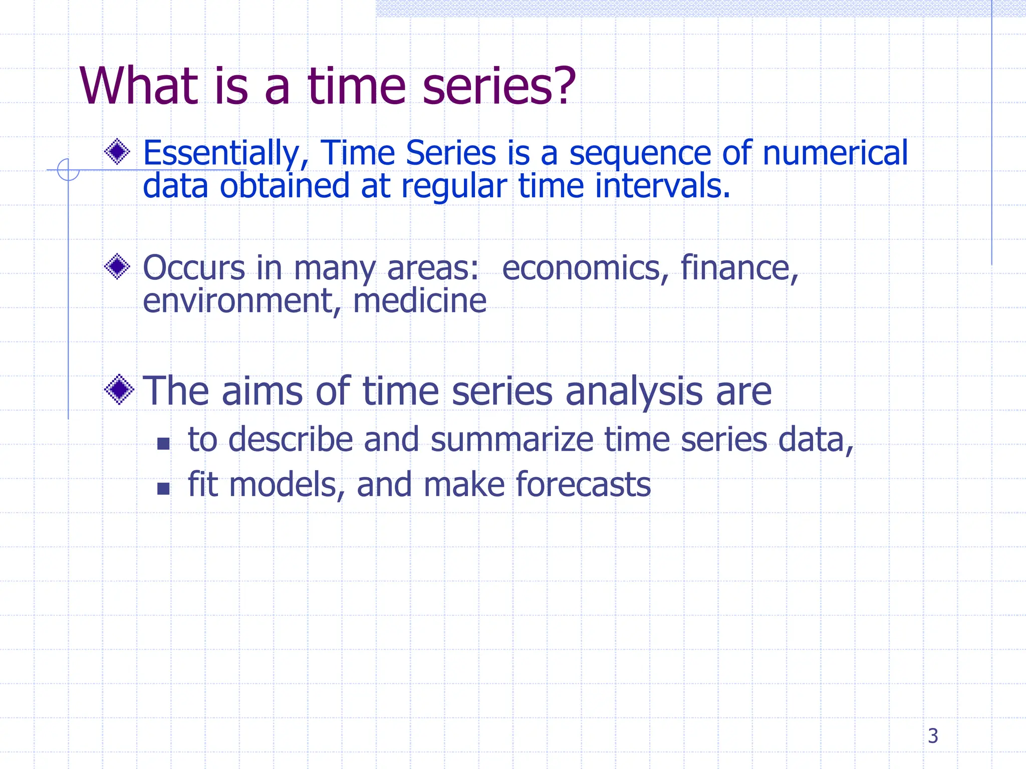
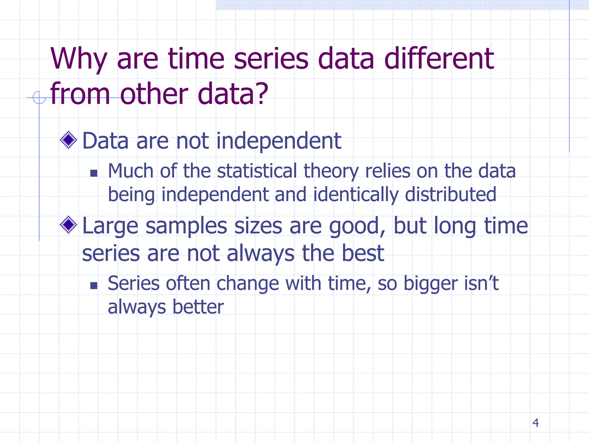
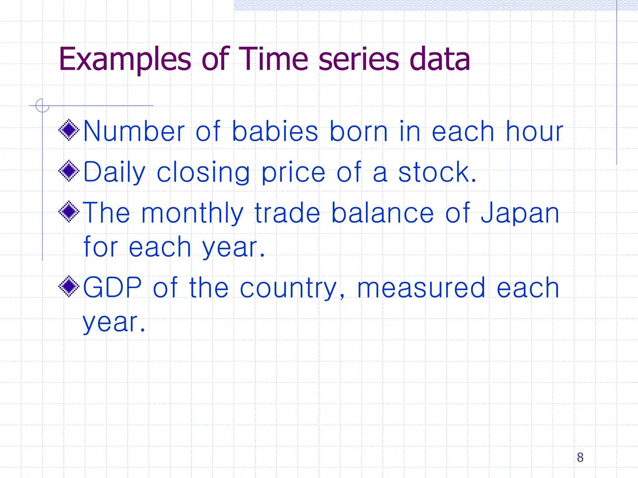
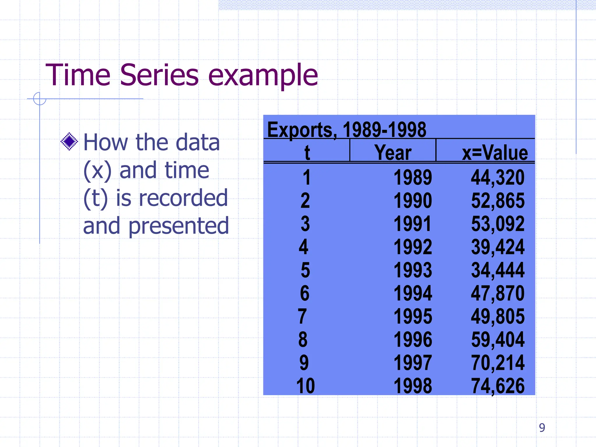
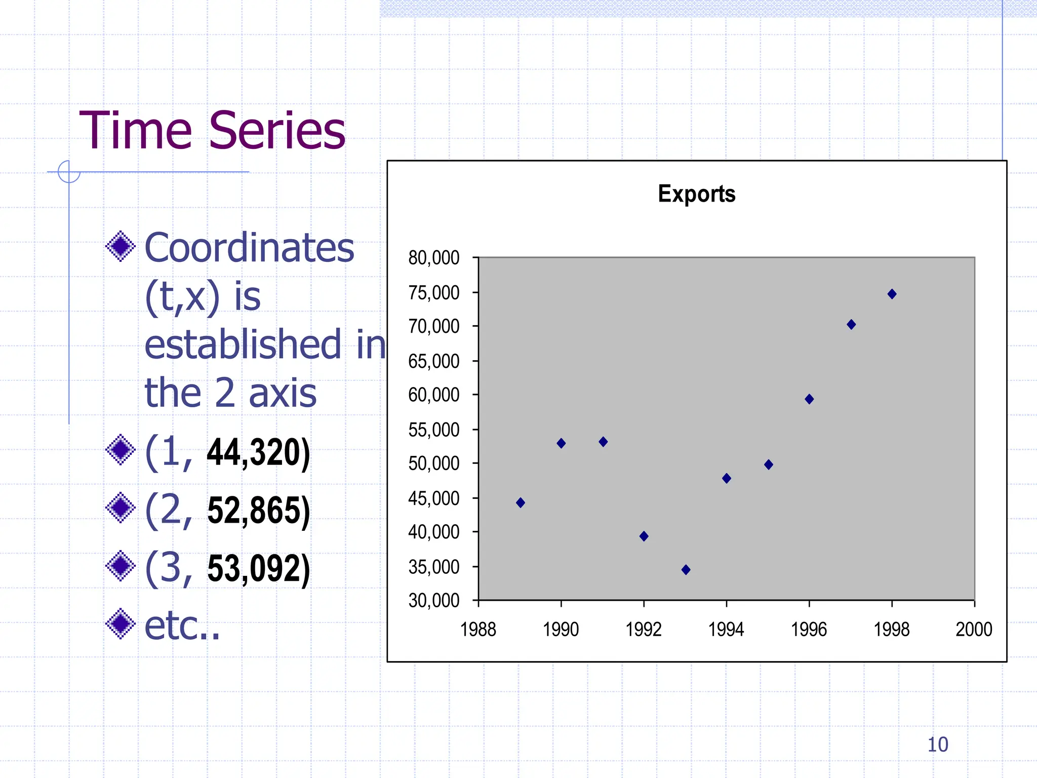
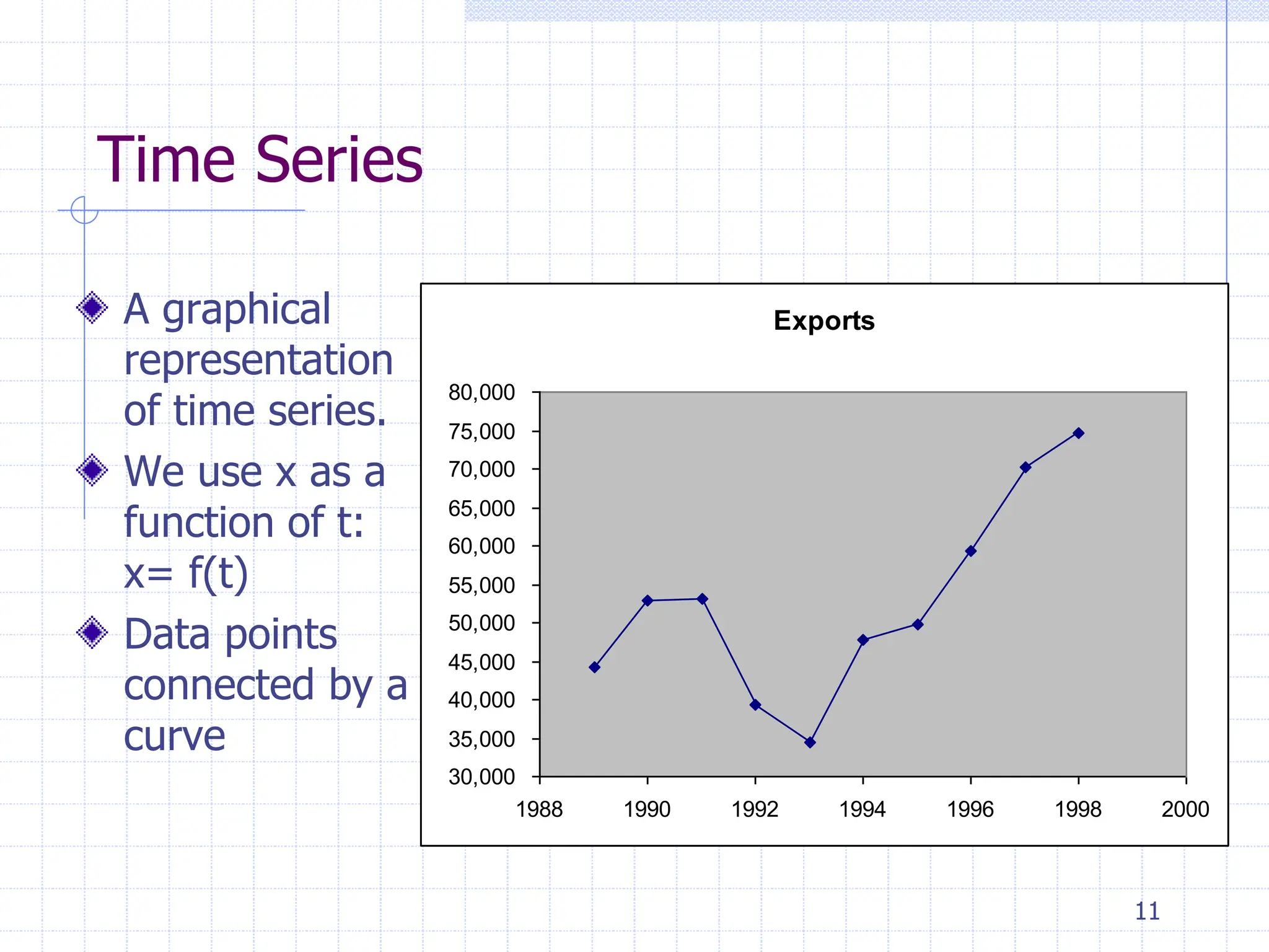
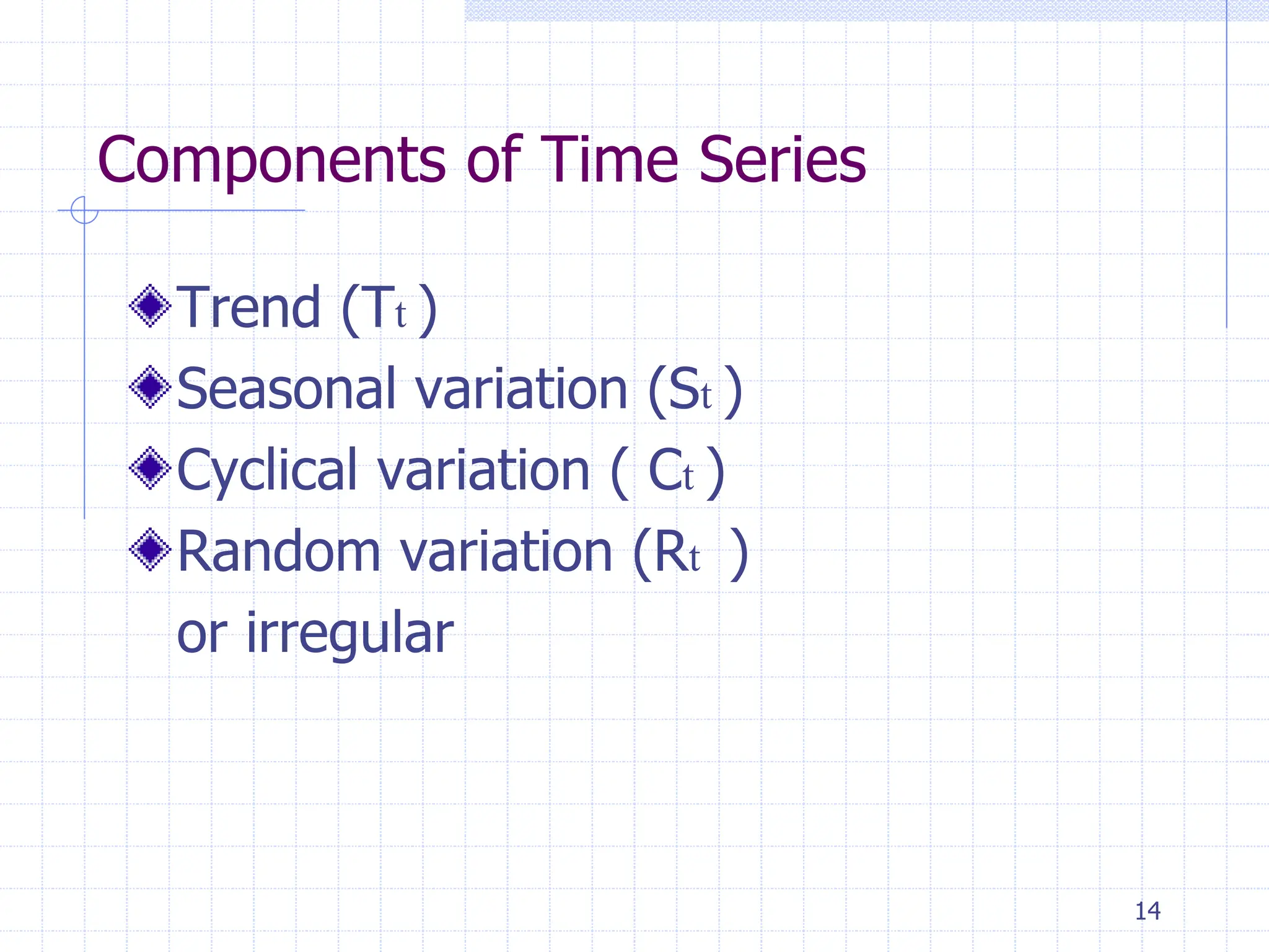
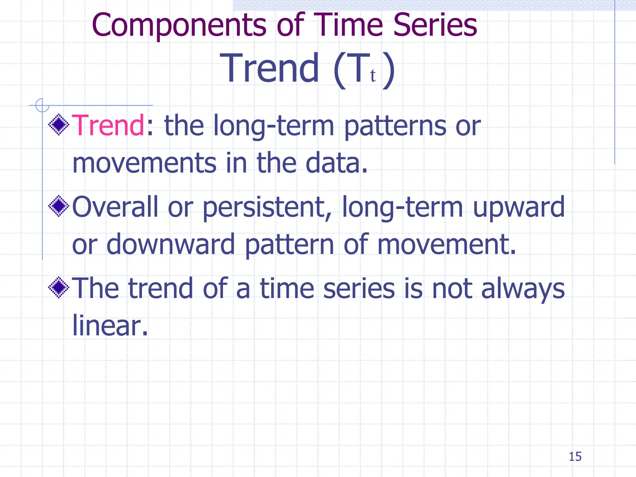
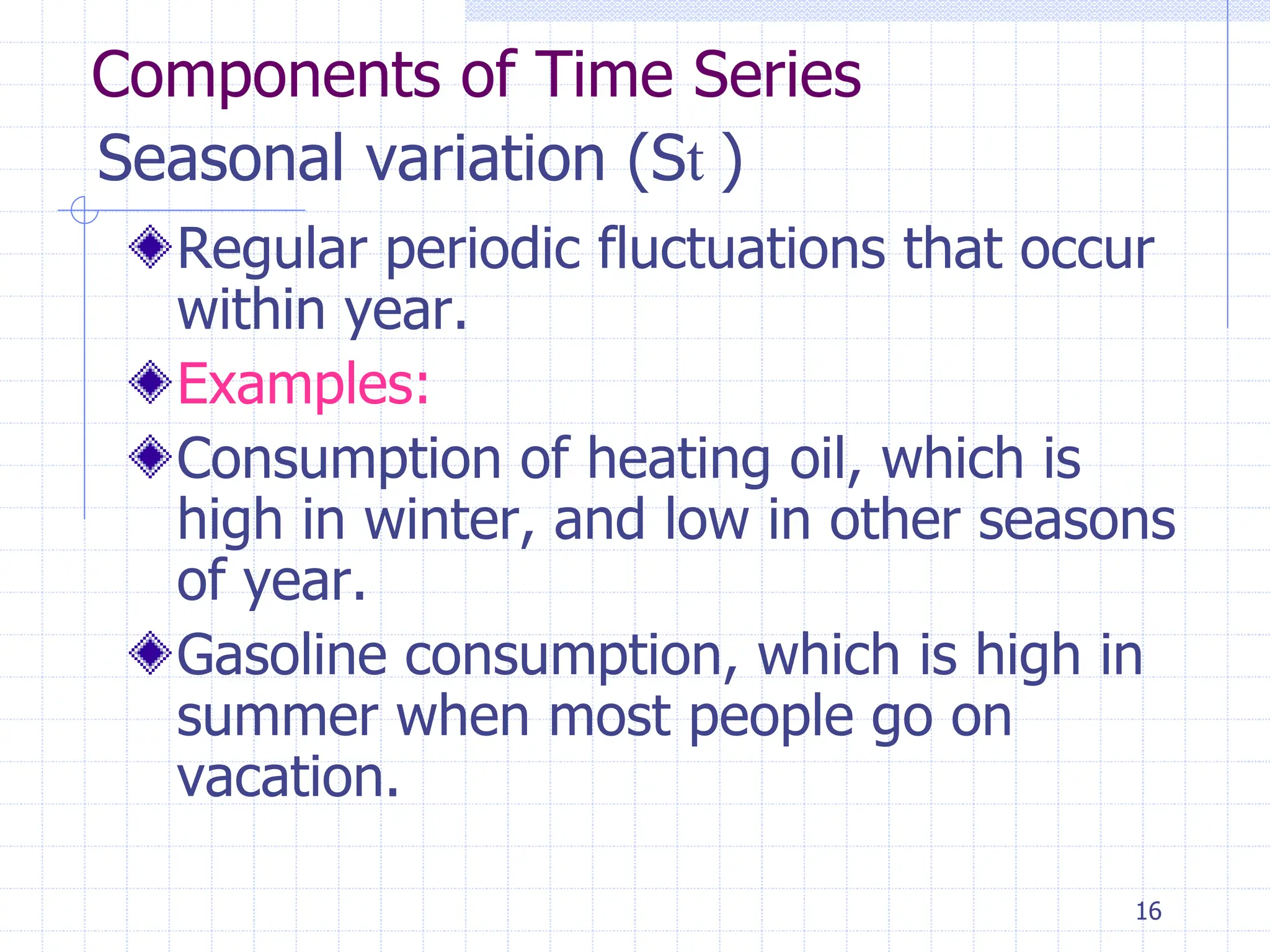
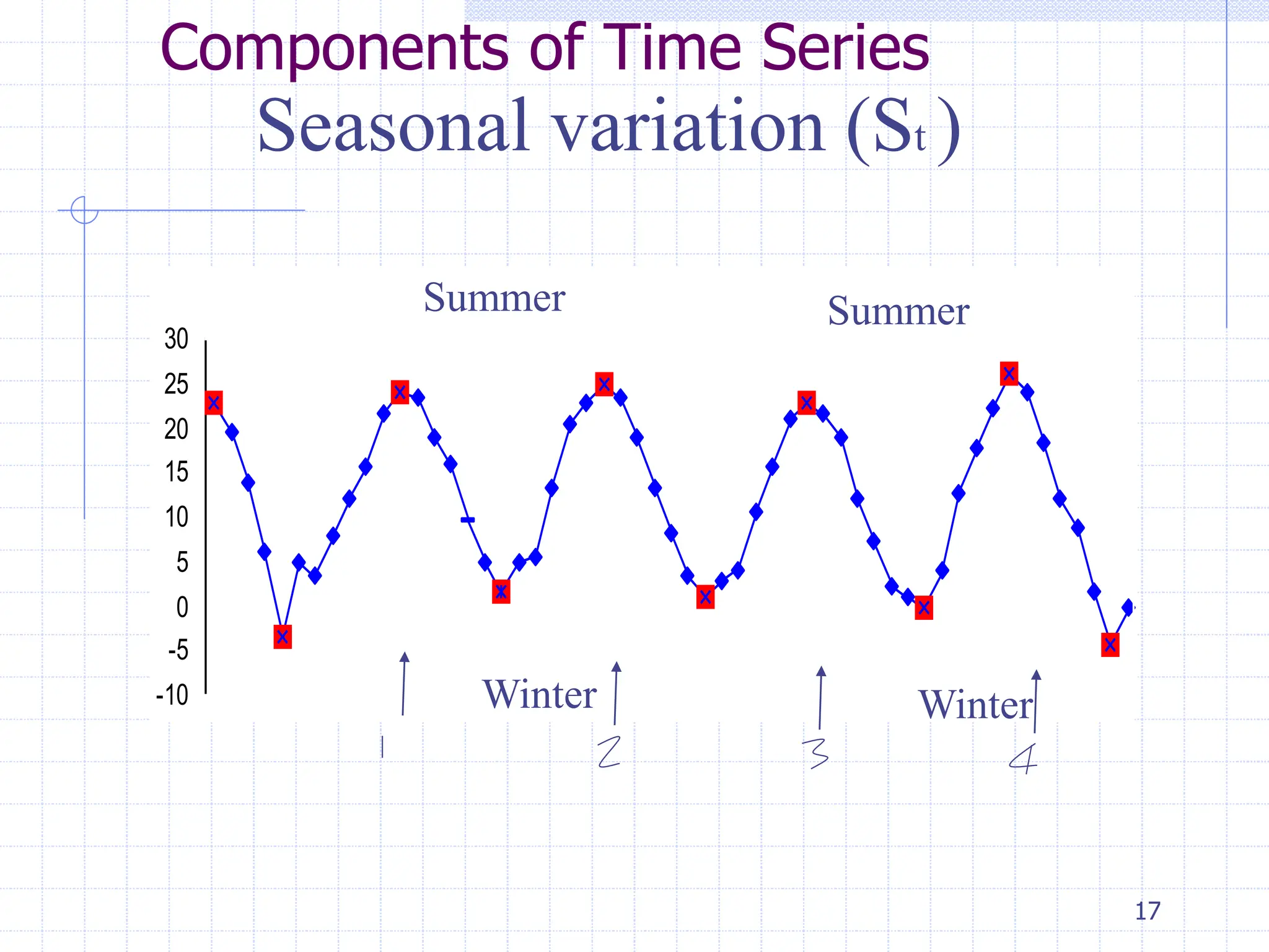
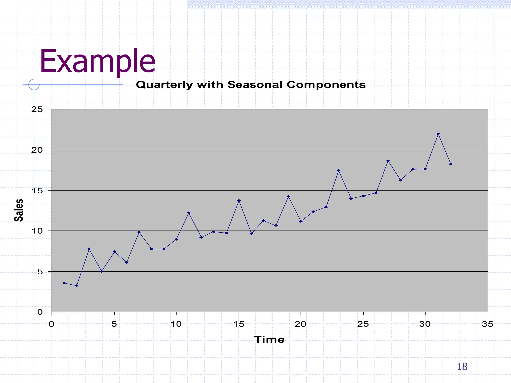
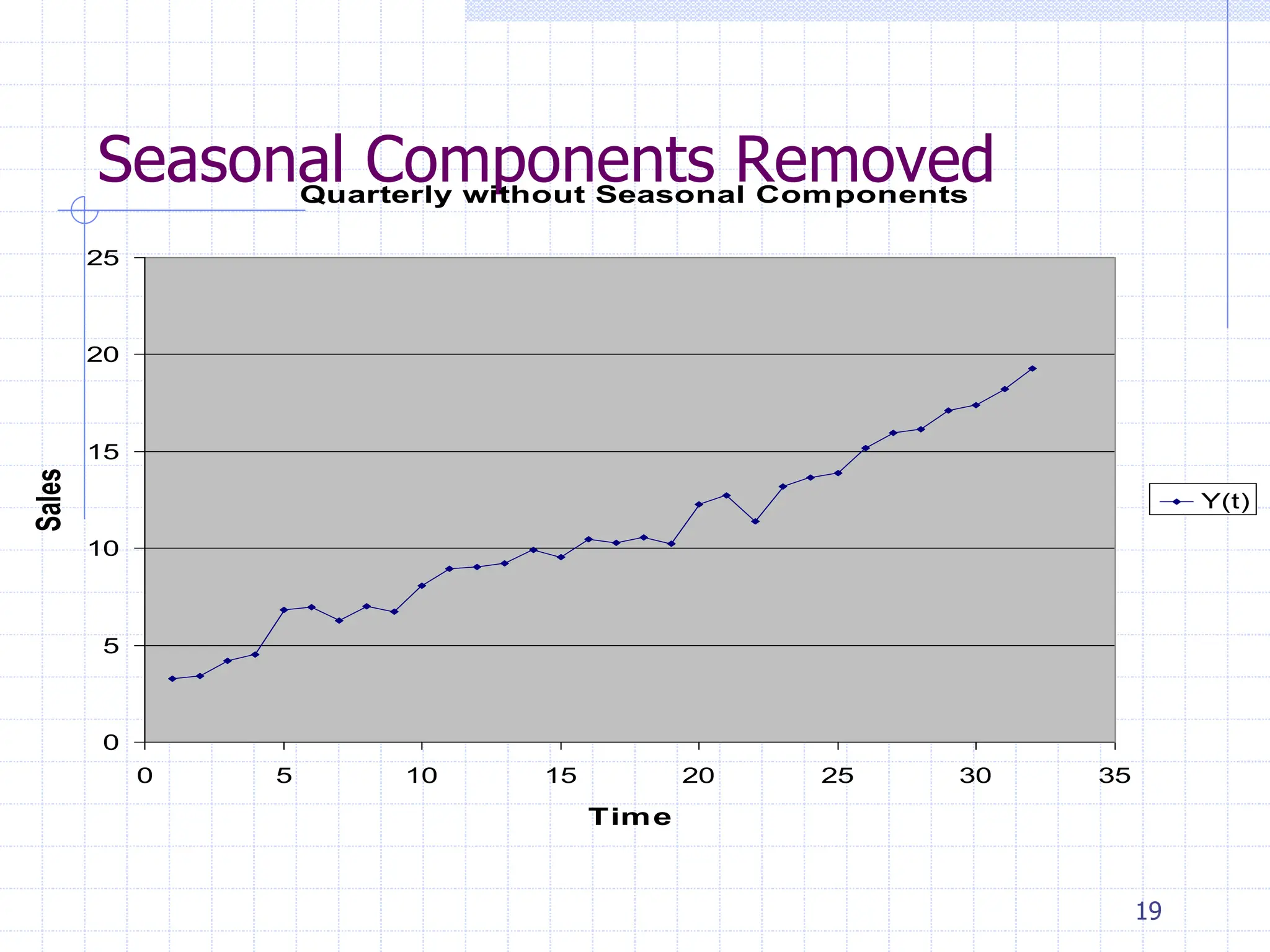
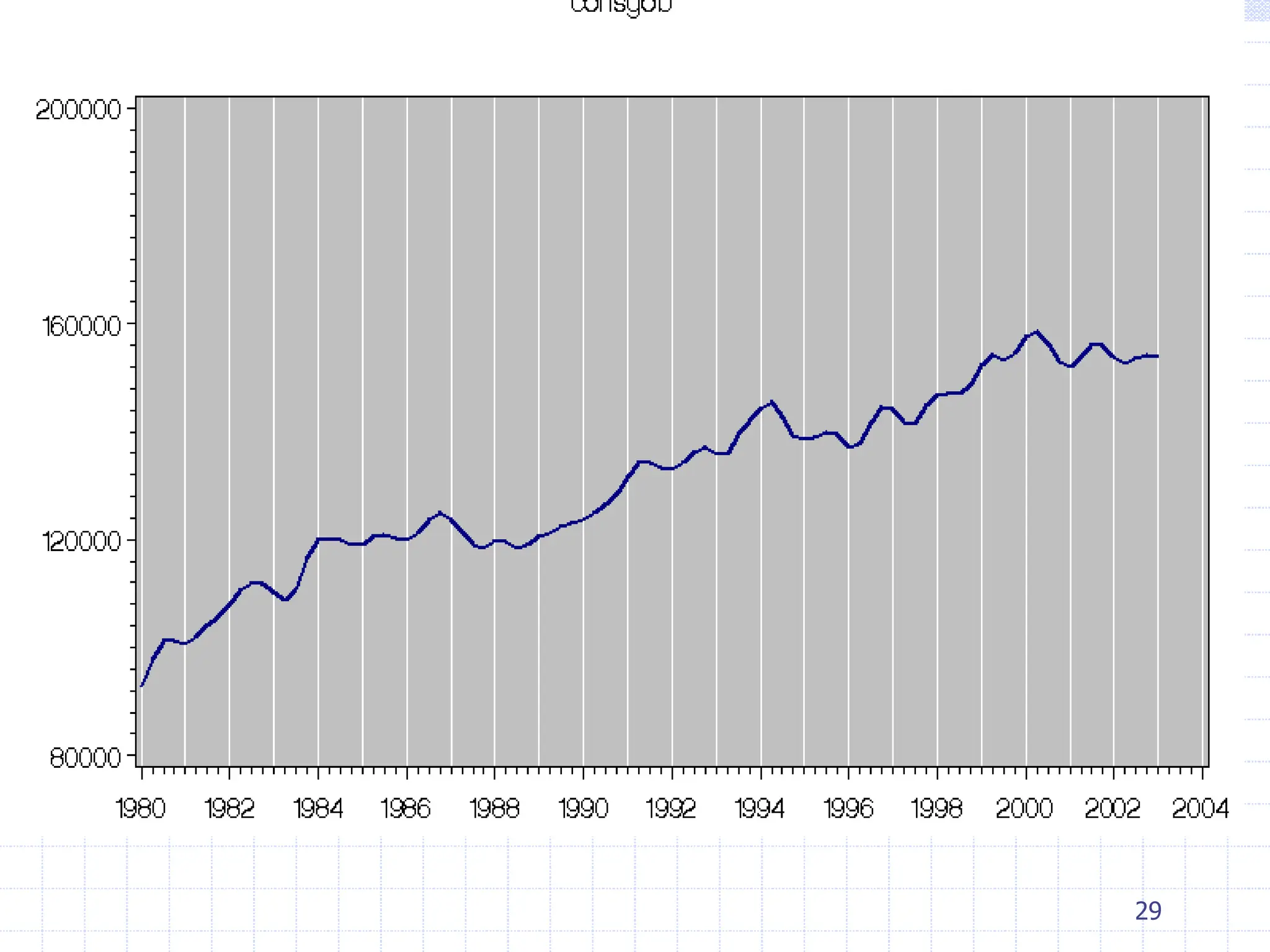
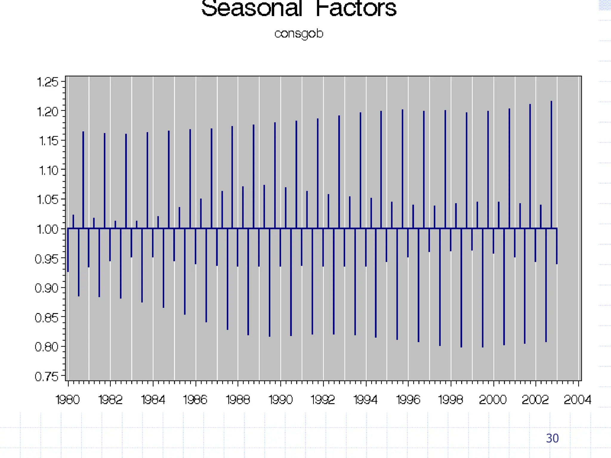
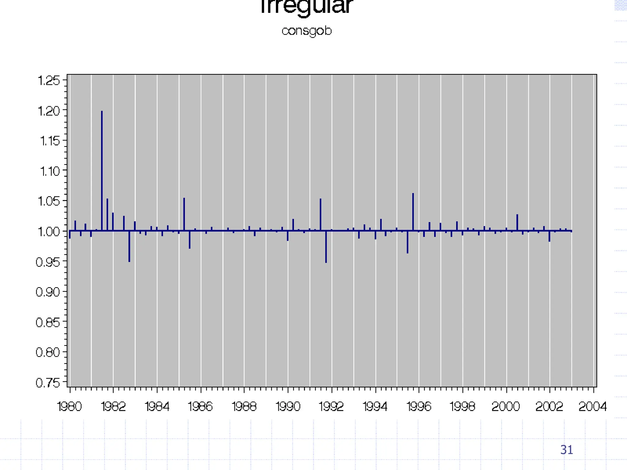
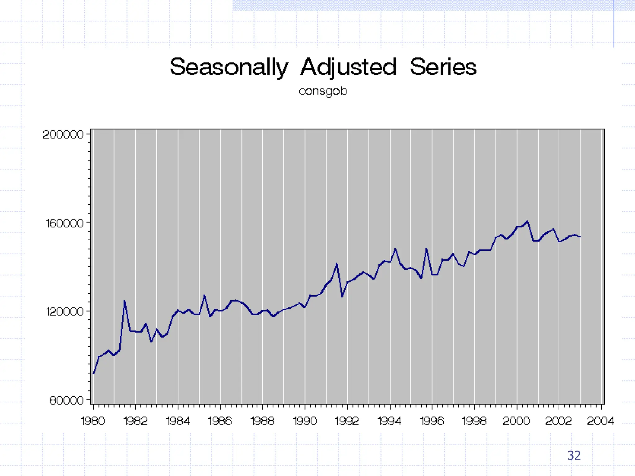
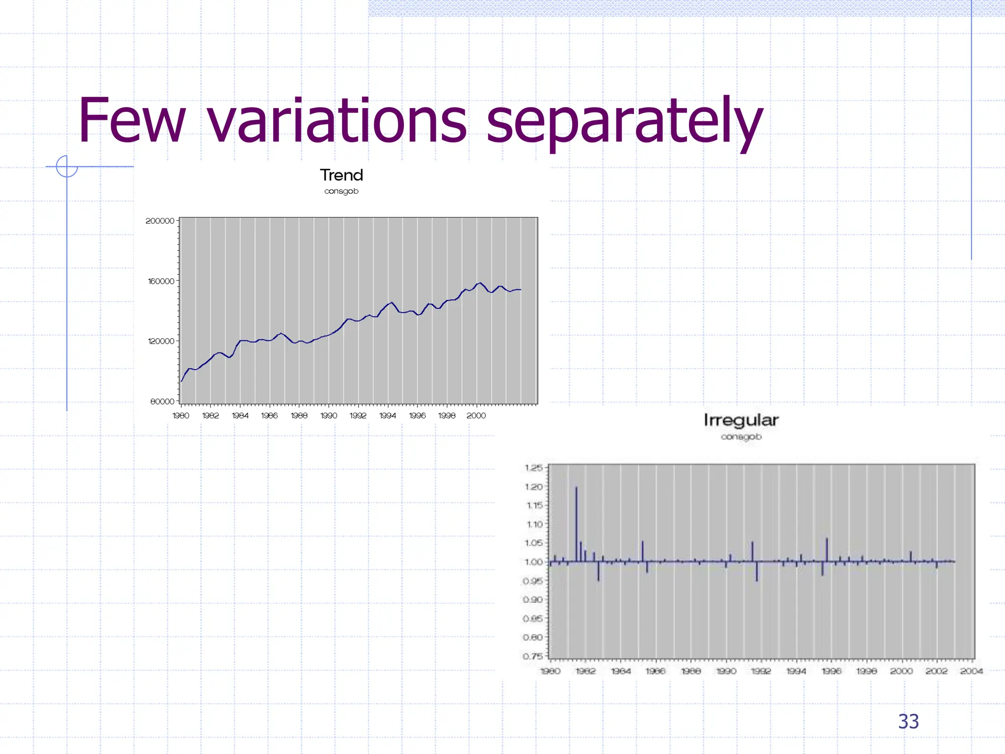
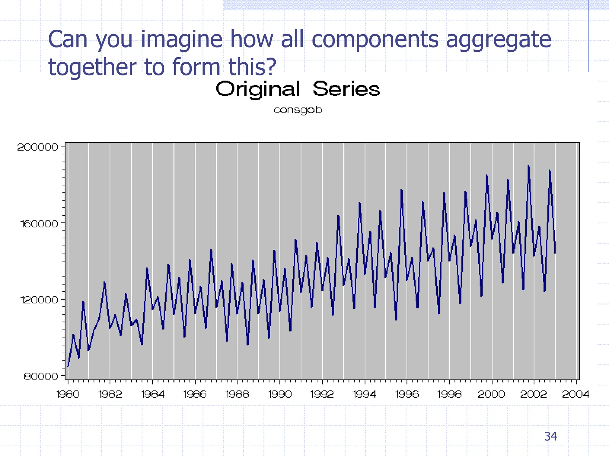
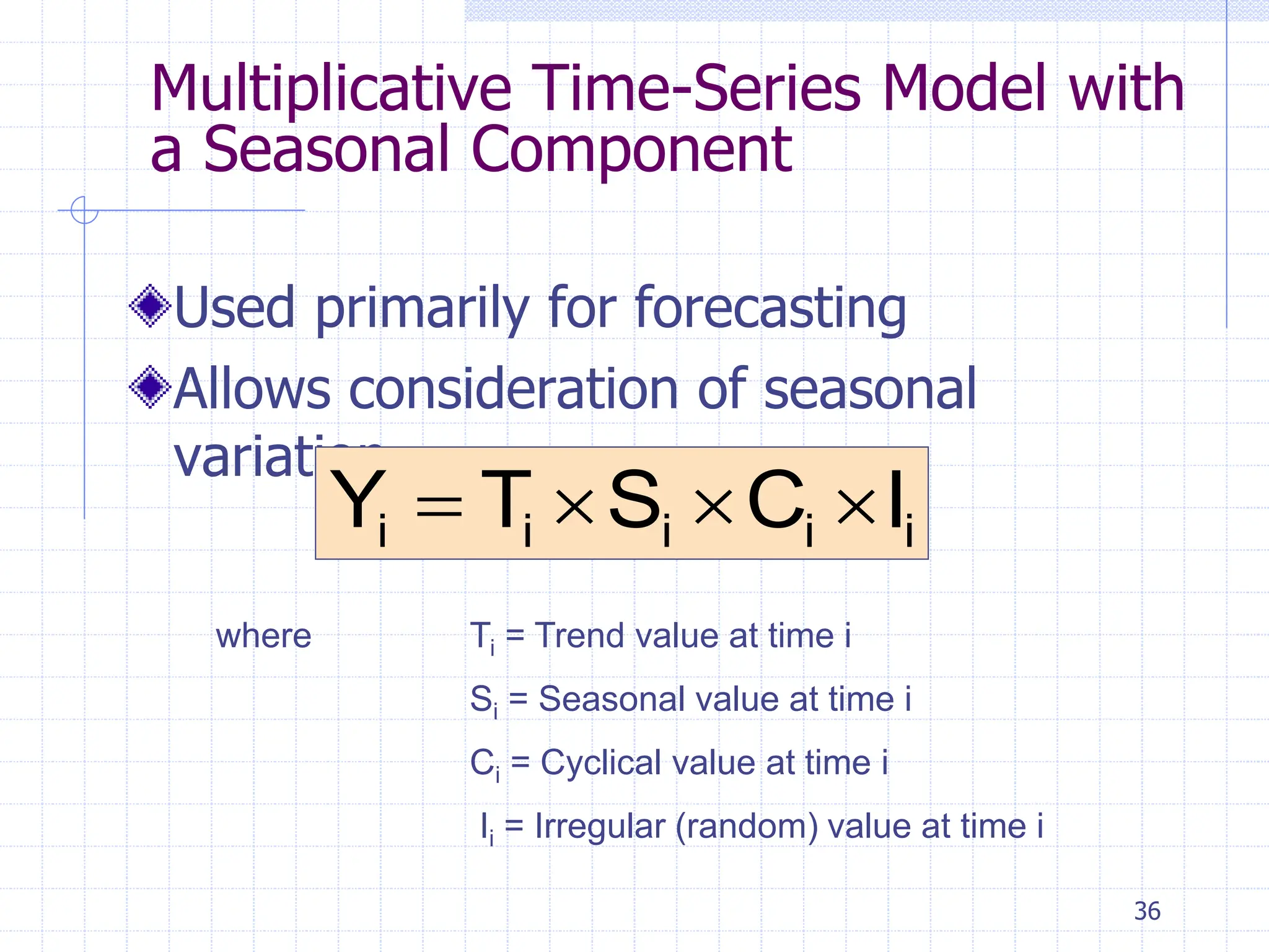
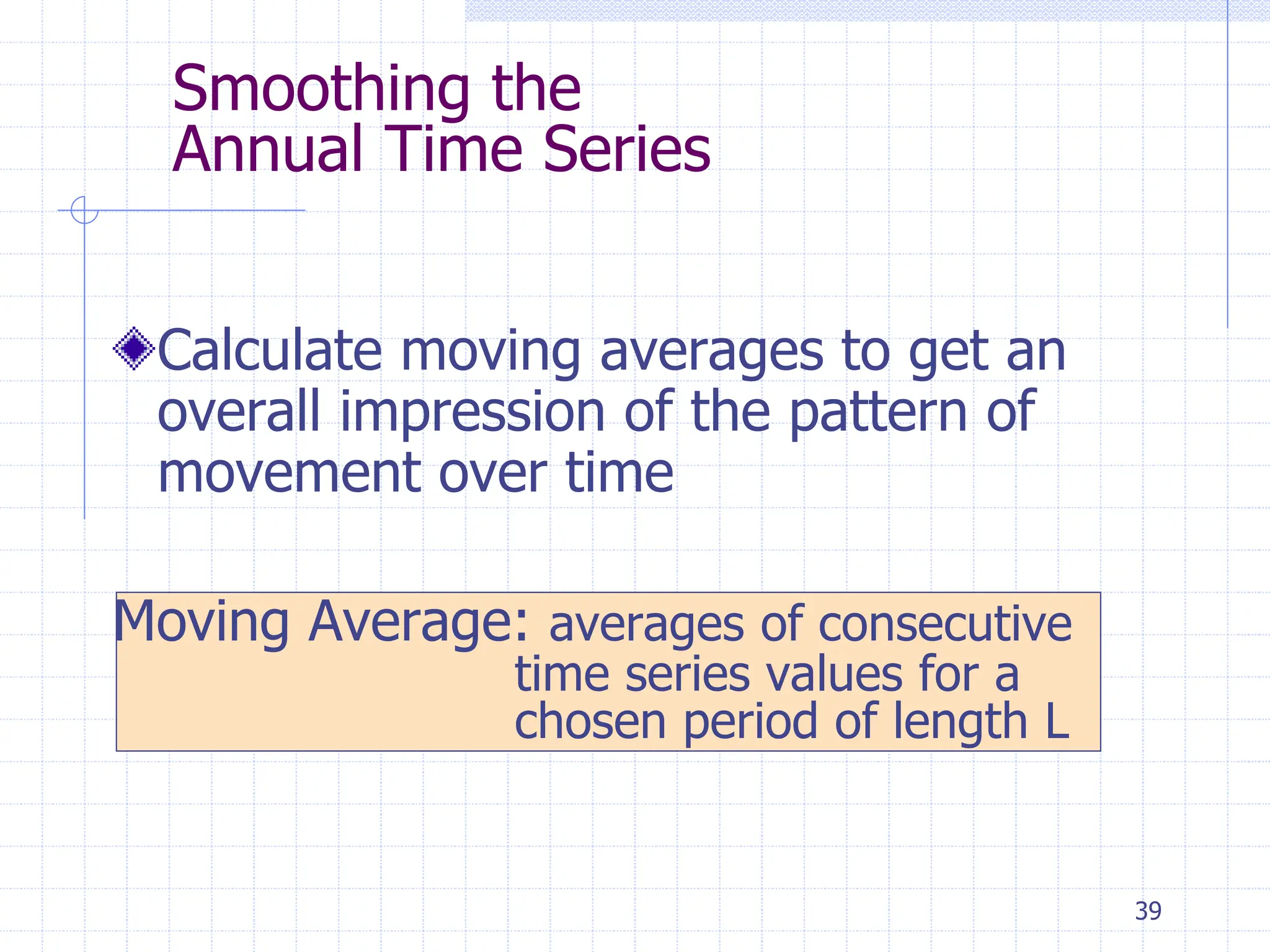
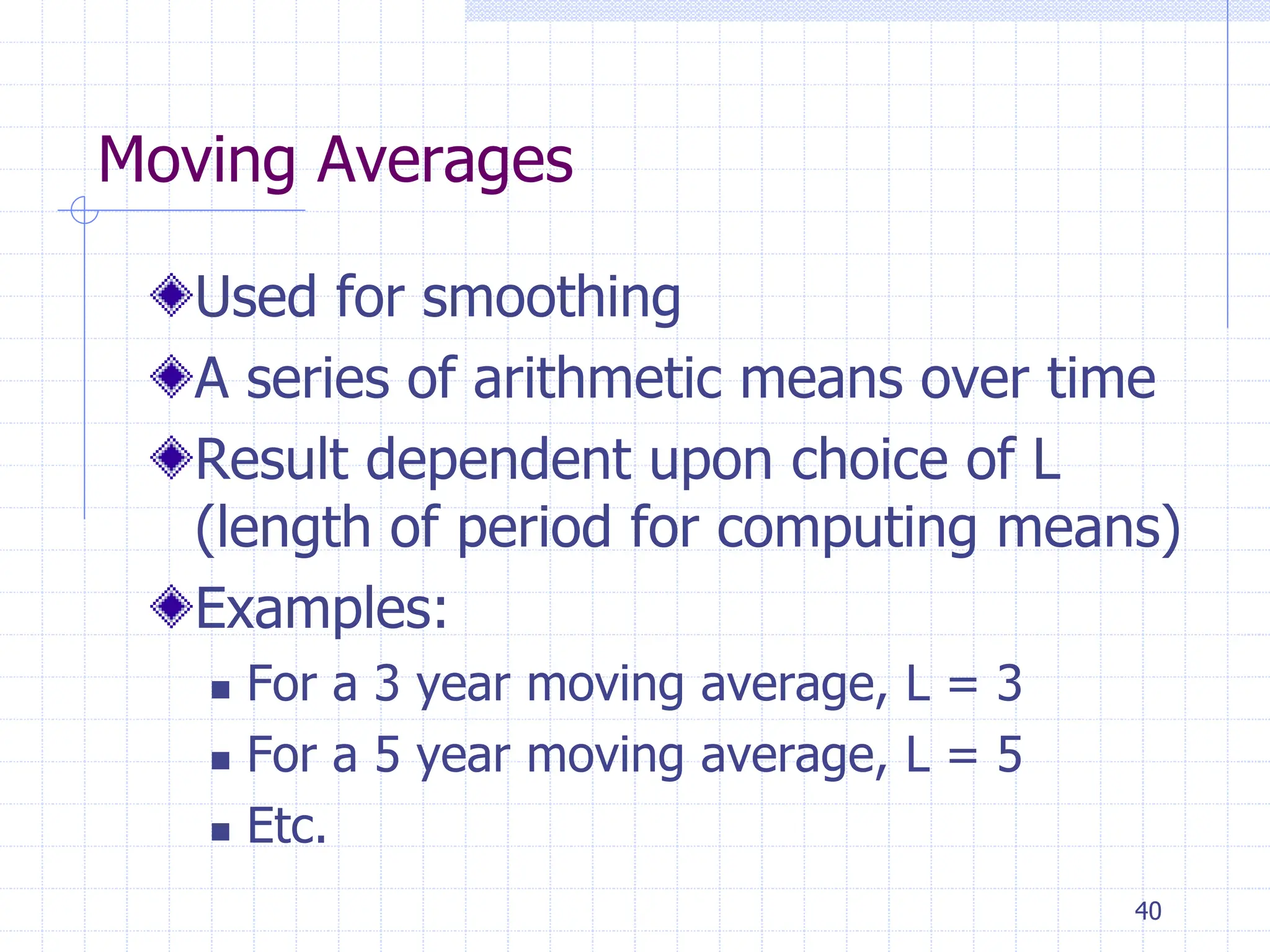
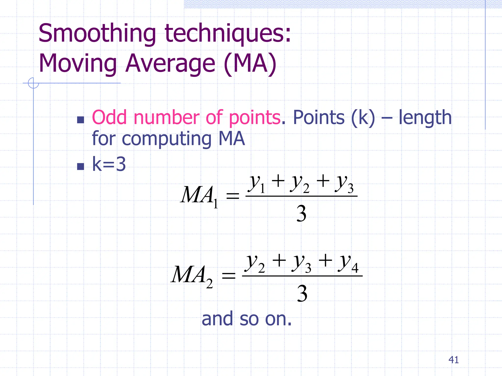
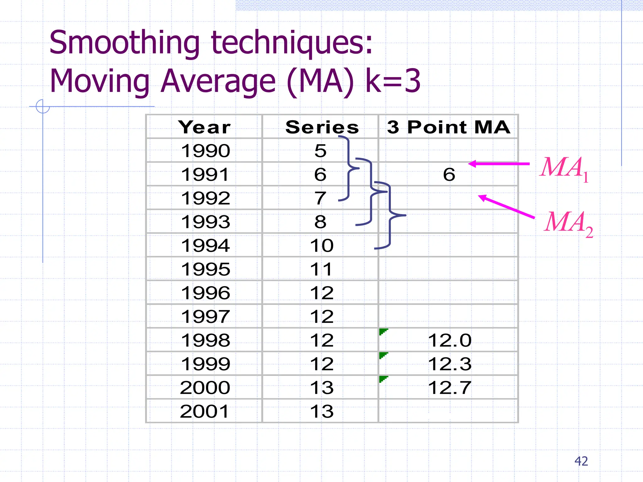
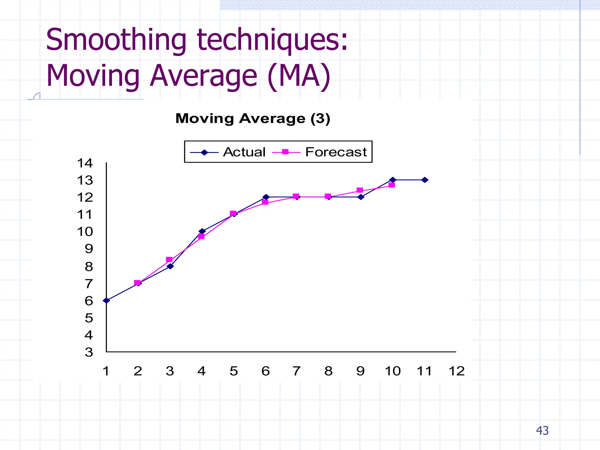
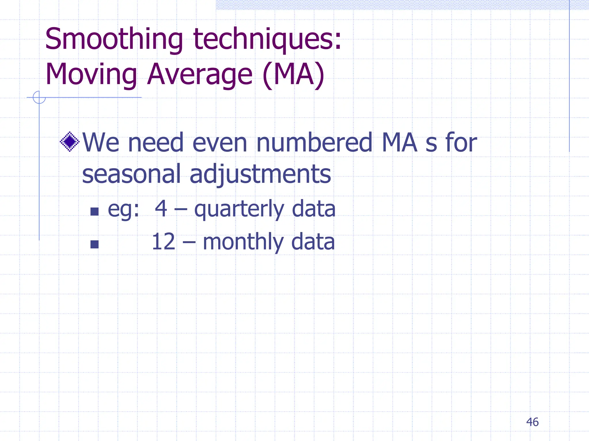
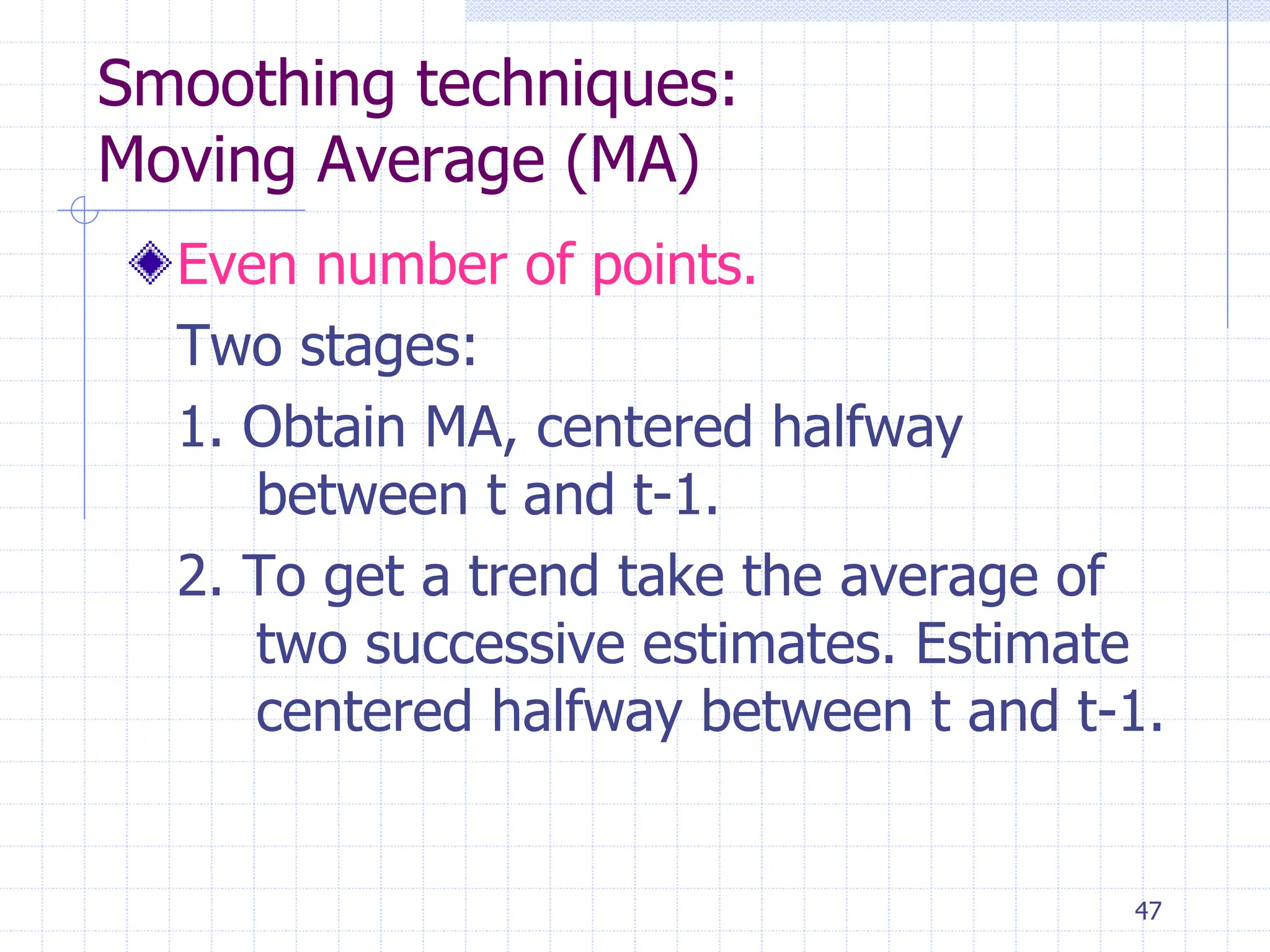
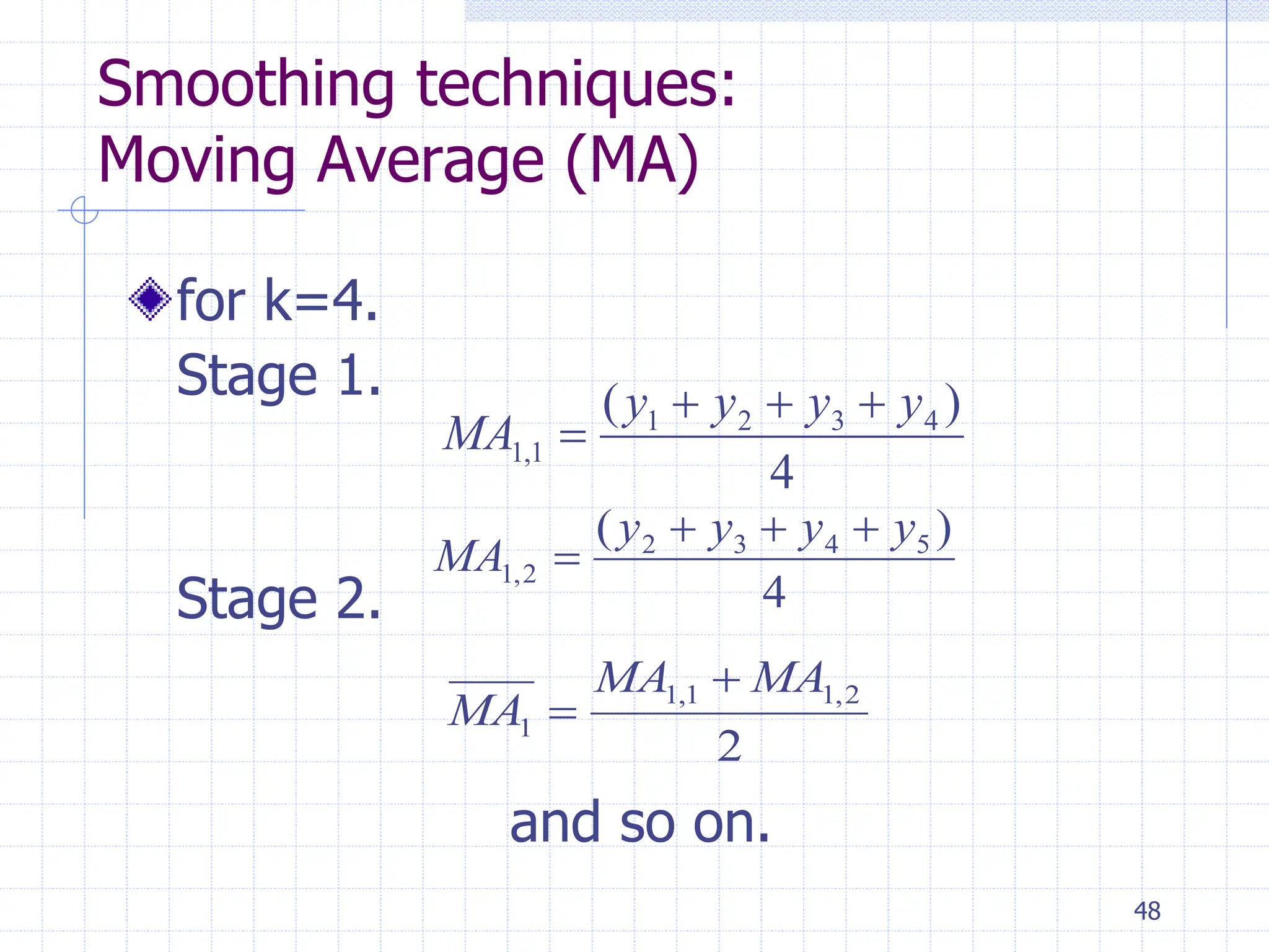
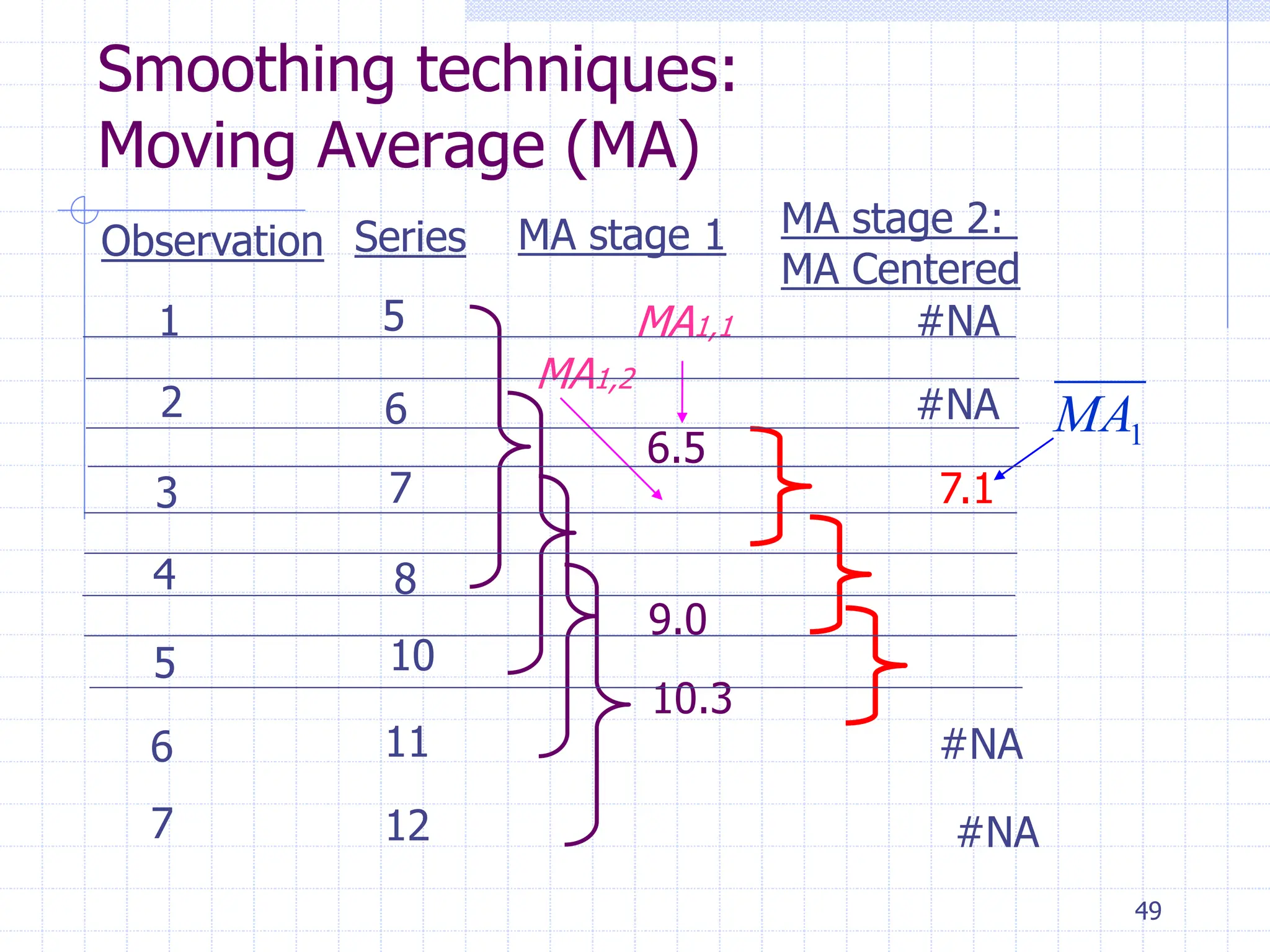
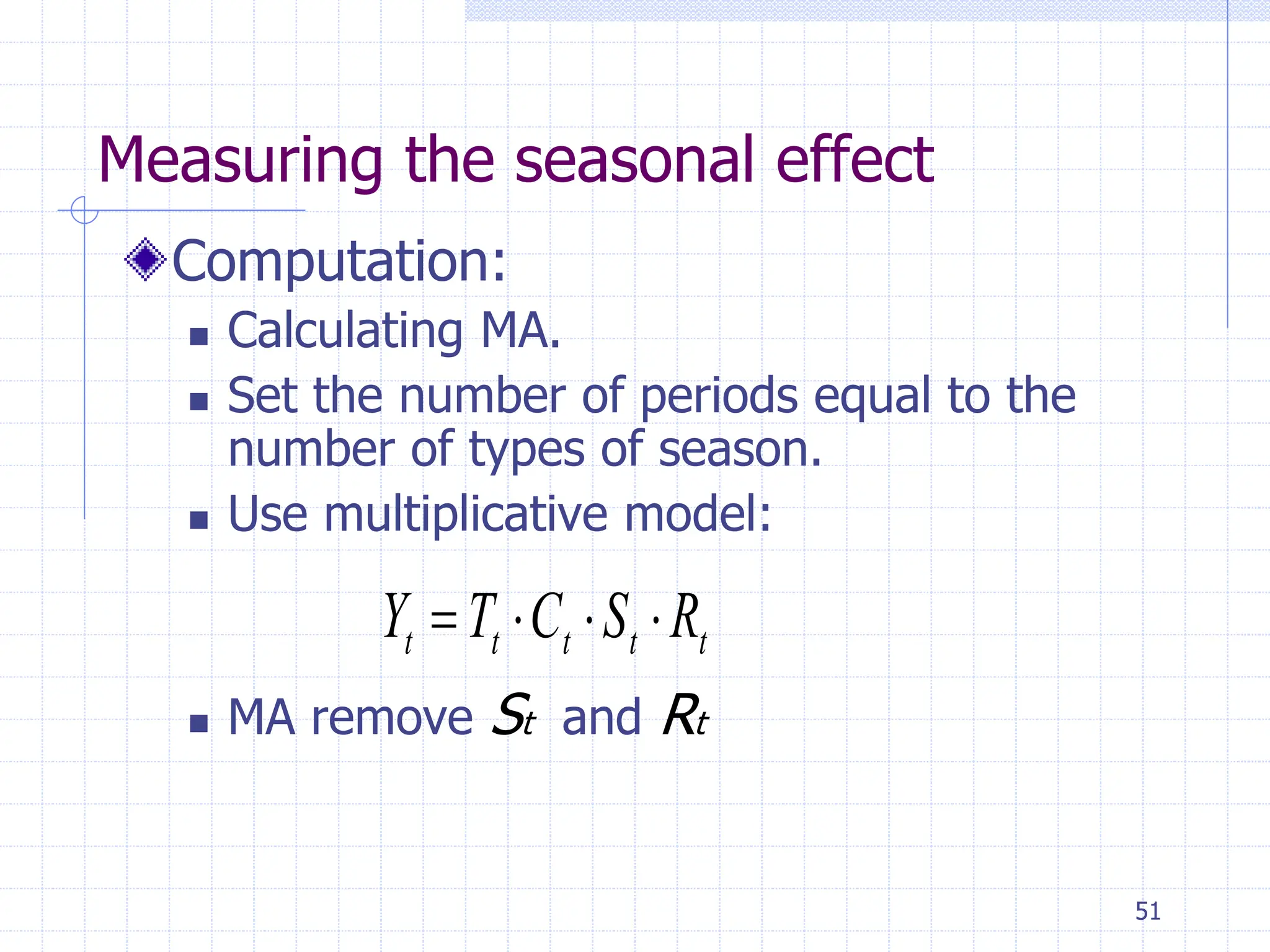
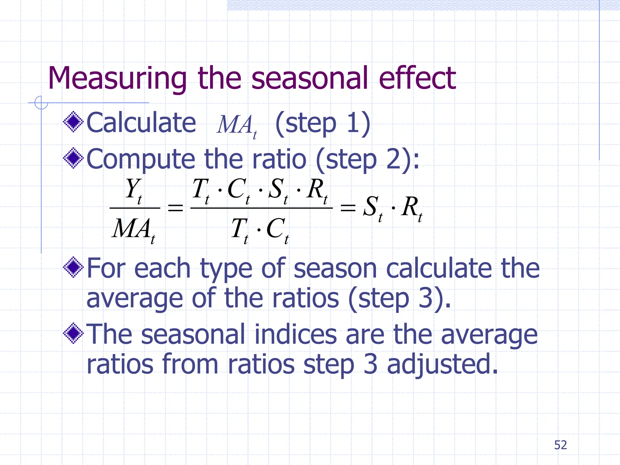
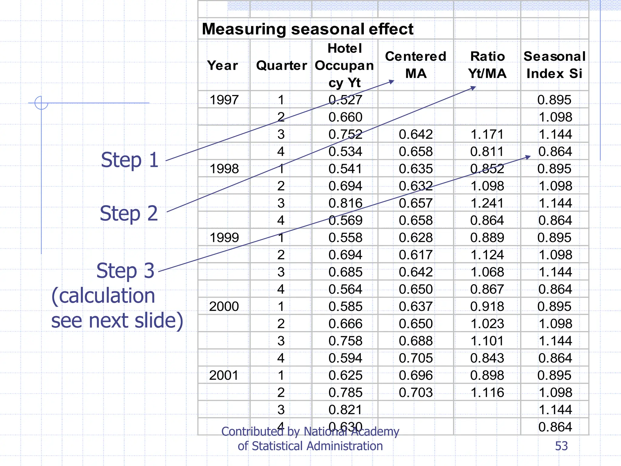
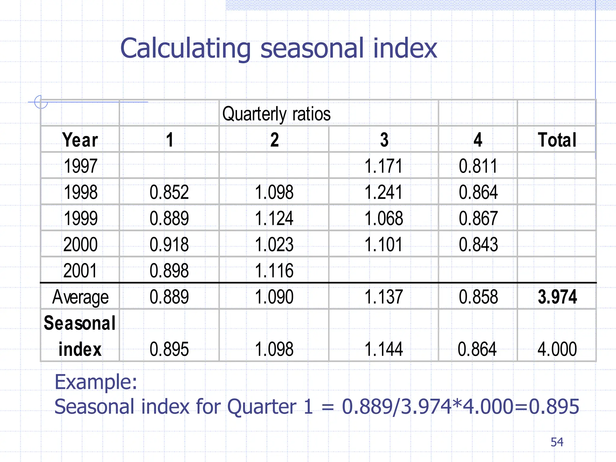
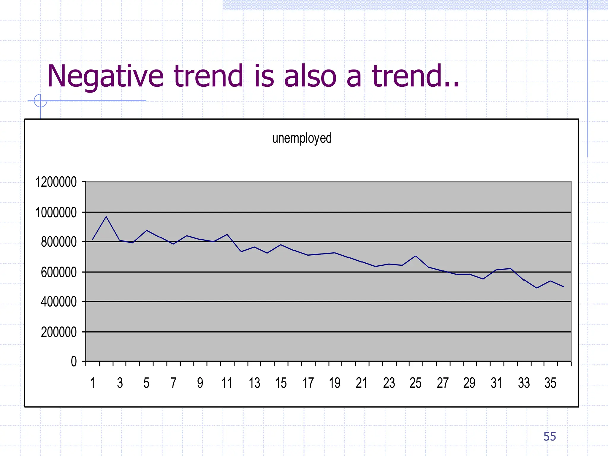
1
Time Series Analysis
2
Module objectives
Introduce time series
Components of time series
Deseasonalising a time series
3
What is a time series?
Essentially, Time Series is a sequence of numerical
data obtained at regular time intervals.
Occurs in many areas: economics, finance,
environment, medicine
The aims of time series analysis are
 to describe and summarize time series data,
 fit models, and make forecasts
4
Why are time series data different
from other data?
Data are not independent
 Much of the statistical theory relies on the data
being independent and identically distributed
Large samples sizes are good, but long time
series are not always the best
 Series often change with time, so bigger isn’t
always better
5
What Are Users Looking for in an
Economic Time Series?
Important features of economic
indicator series include
 Direction
 Turning points
 In addition, we want to see if the
series is increasing/decreasing more
slowly/faster than it was before
6
When should time series analysis
best be used?
We do not assume the existence of deterministic model
governing the behaviour of the system considered.
Instances where deterministic factors are not readily available
and the accuracy of the estimate can be compromised on the
need..(be careful!)
We will only consider univariate time series
7
Forecasting Horizons
Long Term
 5+ years into the future
 R&D, plant location, product planning
 Principally judgement-based
Medium Term
 1 season to 2 years
 Aggregate planning, capacity planning, sales forecasts
 Mixture of quantitative methods and judgement
Short Term
 1 day to 1 year, less than 1 season
 Demand forecasting, staffing levels, purchasing, inventory
levels
 Quantitative methods
8
Examples of Time series data
Number of babies born in each hour
Daily closing price of a stock.
The monthly trade balance of Japan
for each year.
GDP of the country, measured each
year.
9
Time Series example
How the data
(x) and time
(t) is recorded
and presented
Exports, 1989-1998
t Year x=Value
1 1989 44,320
2 1990 52,865
3 1991 53,092
4 1992 39,424
5 1993 34,444
6 1994 47,870
7 1995 49,805
8 1996 59,404
9 1997 70,214
10 1998 74,626
10
Time Series
Coordinates
(t,x) is
established in
the 2 axis
(1, 44,320)
(2, 52,865)
(3, 53,092)
etc..
Exports
30,000
35,000
40,000
45,000
50,000
55,000
60,000
65,000
70,000
75,000
80,000
1988 1990 1992 1994 1996 1998 2000
11
Time Series
A graphical
representation
of time series.
We use x as a
function of t:
x= f(t)
Data points
connected by a
curve
Exports
30,000
35,000
40,000
45,000
50,000
55,000
60,000
65,000
70,000
75,000
80,000
1988 1990 1992 1994 1996 1998 2000
12
Importance of time series analysis
 Understand the past.
What happened over the last years,
months?
 Forecast the future.
Government wants to know future of
unemployment rate, percentage increase in
cost of living etc.
For companies to predict the demand for
their product etc.
13
Time-Series Components
Time-Series
Cyclical
Random
Trend
Seasonal
14
Components of Time Series
Trend (Tt )
Seasonal variation (St )
Cyclical variation ( Ct )
Random variation (Rt )
or irregular
15
Components of Time Series
Trend (Tt )
Trend: the long-term patterns or
movements in the data.
Overall or persistent, long-term upward
or downward pattern of movement.
The trend of a time series is not always
linear.
16
Seasonal variation (St )
Regular periodic fluctuations that occur
within year.
Examples:
Consumption of heating oil, which is
high in winter, and low in other seasons
of year.
Gasoline consumption, which is high in
summer when most people go on
vacation.
Components of Time Series
17
-10
-5
0
5
10
15
20
25
30
Seasonal variation (St )
Summer
Winter Winter
Summer
Components of Time Series
18
Example
Quarterly with Seasonal Components
0
5
10
15
20
25
0 5 10 15 20 25 30 35
Time
Sales
19
Seasonal Components Removed
Quarterly without Seasonal Components
0
5
10
15
20
25
0 5 10 15 20 25 30 35
Time
Sales
Y(t)
20
Why Do Users Want Seasonally
Adjusted Data?
Seasonal movements can make features
difficult or impossible to see
21
Causes of Seasonal Effects
Possible causes are
 Natural factors
 Administrative or legal measures
 Social/cultural/religious traditions
(e.g., fixed holidays, timing of
vacations)
22
Components of Time Series
Cyclical variation ( Ct )
• Cyclical variations are similar to seasonal
variations. Cycles are often irregular both in
height of peak and duration.
• Examples:
• Long-term product demand cycles.
• Cycles in the monetary and financial
sectors. (Important for economists!)
23
Cyclical Component
Long-term wave-like patterns
Regularly occur but may vary in length
Often measured peak to peak or trough
to trough
Sales
1 Cycle
Year
24
Irregular Component
Unpredictable, random, “residual”
fluctuations
Due to random variations of
 Nature
 Accidents or unusual events
“Noise” in the time series
25
Causes of Irregular Effects
Possible causes
 Unseasonable weather/natural disasters
 Strikes
 Sampling error
 Nonsampling error
26
Classical Decomposition
One method of describing a time series
Decompose the series into various components
 Trend – long term movements in the level of the series
 Seasonal effects – cyclical fluctuations reasonably stable in
terms of annual timing (including moving holidays and
working day effects)
 Cycles – cyclical fluctuations longer than a year
 Irregular – other random or short-term unpredictable
fluctuations
27
Not easy to understand the pattern!
28
Our aim
is to understand and identify different
variations so that we can easily predict
the future variations separately and
combine together
Look how the above complicated series
could be understood as follows
separately
29
30
31
32
Few variations separately
33
34
Can you imagine how all components aggregate
together to form this?
35
Multiplicative Time-Series Model for
Annual Data
Used primarily for forecasting
Observed value in time series is the
product of components
where Ti = Trend value at year i
Ci = Cyclical value at year i
Ii = Irregular (random) value at year i
i
i
i
i I
C
T
Y 


36
Multiplicative Time-Series Model with
a Seasonal Component
Used primarily for forecasting
Allows consideration of seasonal
variation
where Ti = Trend value at time i
Si = Seasonal value at time i
Ci = Cyclical value at time i
Ii = Irregular (random) value at time i
i
i
i
i
i I
C
S
T
Y 



37
Smoothing techniques
Smoothing helps to see overall patterns
in time series data.
Smoothing techniques smooth or “iron”
out variation to get the overall picture.
There are several smoothing techniques
of time series.
38
Smoothing techniques
We will study :
Moving average.
Exponential smoothing
39
Smoothing the
Annual Time Series
Calculate moving averages to get an
overall impression of the pattern of
movement over time
Moving Average: averages of consecutive
time series values for a
chosen period of length L
40
Moving Averages
Used for smoothing
A series of arithmetic means over time
Result dependent upon choice of L
(length of period for computing means)
Examples:
 For a 3 year moving average, L = 3
 For a 5 year moving average, L = 5
 Etc.
41
Smoothing techniques:
Moving Average (MA)
 Odd number of points. Points (k) – length
for computing MA
 k=3
and so on.
3
3
2
1
1
y
y
y
MA



3
4
3
2
2
y
y
y
MA



42
Smoothing techniques:
Moving Average (MA) k=3
Year Series 3 Point MA
1990 5
1991 6 6
1992 7
1993 8
1994 10
1995 11
1996 12
1997 12
1998 12 12.0
1999 12 12.3
2000 13 12.7
2001 13
1
MA
2
MA
43
Smoothing techniques:
Moving Average (MA)
Moving Average (3)
3
4
5
6
7
8
9
10
11
12
13
14
1 2 3 4 5 6 7 8 9 10 11 12
Actual Forecast
44
Smoothing techniques:
Moving Average (MA) k=5
Year Series 5 Point MA
1990 5
1991 6
1992 7 7.2
1993 8
1994 10
1995 11
1996 12
1997 12
1998 12
1999 12 12.4
2000 13
2001 13
45
Smoothing techniques:
Moving Average (MA)
Moving Average (5)
0
2
4
6
8
10
12
14
1 2 3 4 5 6 7 8 9 10 11
Actual Forecast
46
Smoothing techniques:
Moving Average (MA)
We need even numbered MA s for
seasonal adjustments
 eg: 4 – quarterly data
 12 – monthly data
47
Smoothing techniques:
Moving Average (MA)
Even number of points.
Two stages:
1. Obtain MA, centered halfway
between t and t-1.
2. To get a trend take the average of
two successive estimates. Estimate
centered halfway between t and t-1.
48
Smoothing techniques:
Moving Average (MA)
for k=4.
Stage 1.
Stage 2.
and so on.
4
)
( 4
3
2
1
1
,
1
y
y
y
y
MA




4
)
( 5
4
3
2
2
,
1
y
y
y
y
MA




2
2
,
1
1
,
1
1
MA
MA
MA


49
Smoothing techniques:
Moving Average (MA)
Observation Series MA stage 1 MA stage 2:
MA Centered
1
2
3
4
5
6
7
5
6
7
8
10
11
12
6.5
9.0
10.3
7.1
#NA
#NA
#NA
#NA
MA1,1
MA1,2
1
MA
50
Measuring the seasonal effect
To measure seasonal effect construct
seasonal indices.
Seasonal indices is a degree to which
the seasons differ from one another.
Requirement: time series should be
sufficiently long to allow to observe
seasonal fluctuations.
51
Measuring the seasonal effect
Computation:
 Calculating MA.
 Set the number of periods equal to the
number of types of season.
 Use multiplicative model:
 MA remove St and Rt
t
t
t
t
t R
S
C
T
Y 



52
Measuring the seasonal effect
Calculate (step 1)
Compute the ratio (step 2):
For each type of season calculate the
average of the ratios (step 3).
The seasonal indices are the average
ratios from ratios step 3 adjusted.
t
t
t
t
t
t
t
t
t
t
R
S
C
T
R
S
C
T
MA
Y







t
MA
53
Measuring seasonal effect
Year Quarter
Hotel
Occupan
cy Yt
Centered
MA
Ratio
Yt/MA
Seasonal
Index Si
1997 1 0.527 0.895
2 0.660 1.098
3 0.752 0.642 1.171 1.144
4 0.534 0.658 0.811 0.864
1998 1 0.541 0.635 0.852 0.895
2 0.694 0.632 1.098 1.098
3 0.816 0.657 1.241 1.144
4 0.569 0.658 0.864 0.864
1999 1 0.558 0.628 0.889 0.895
2 0.694 0.617 1.124 1.098
3 0.685 0.642 1.068 1.144
4 0.564 0.650 0.867 0.864
2000 1 0.585 0.637 0.918 0.895
2 0.666 0.650 1.023 1.098
3 0.758 0.688 1.101 1.144
4 0.594 0.705 0.843 0.864
2001 1 0.625 0.696 0.898 0.895
2 0.785 0.703 1.116 1.098
3 0.821 1.144
4 0.630 0.864
Step 1
Step 2
Step 3
(calculation
see next slide)
Contributed by National Academy
of Statistical Administration
54
Quarterly ratios
Year 1 2 3 4 Total
1997 1.171 0.811
1998 0.852 1.098 1.241 0.864
1999 0.889 1.124 1.068 0.867
2000 0.918 1.023 1.101 0.843
2001 0.898 1.116
Average 0.889 1.090 1.137 0.858 3.974
Seasonal
index 0.895 1.098 1.144 0.864 4.000
Calculating seasonal index
Example:
Seasonal index for Quarter 1 = 0.889/3.974*4.000=0.895
55
Negative trend is also a trend..
unemployed
0
200000
400000
600000
800000
1000000
1200000
1 3 5 7 9 11 13 15 17 19 21 23 25 27 29 31 33 35

Enterprise_Planning_TimeSeries_And_Components

  • 1.
  • 2.
    2 Module objectives Introduce timeseries Components of time series Deseasonalising a time series
  • 3.
    3 What is atime series? Essentially, Time Series is a sequence of numerical data obtained at regular time intervals. Occurs in many areas: economics, finance, environment, medicine The aims of time series analysis are  to describe and summarize time series data,  fit models, and make forecasts
  • 4.
    4 Why are timeseries data different from other data? Data are not independent  Much of the statistical theory relies on the data being independent and identically distributed Large samples sizes are good, but long time series are not always the best  Series often change with time, so bigger isn’t always better
  • 5.
    5 What Are UsersLooking for in an Economic Time Series? Important features of economic indicator series include  Direction  Turning points  In addition, we want to see if the series is increasing/decreasing more slowly/faster than it was before
  • 6.
    6 When should timeseries analysis best be used? We do not assume the existence of deterministic model governing the behaviour of the system considered. Instances where deterministic factors are not readily available and the accuracy of the estimate can be compromised on the need..(be careful!) We will only consider univariate time series
  • 7.
    7 Forecasting Horizons Long Term 5+ years into the future  R&D, plant location, product planning  Principally judgement-based Medium Term  1 season to 2 years  Aggregate planning, capacity planning, sales forecasts  Mixture of quantitative methods and judgement Short Term  1 day to 1 year, less than 1 season  Demand forecasting, staffing levels, purchasing, inventory levels  Quantitative methods
  • 8.
    8 Examples of Timeseries data Number of babies born in each hour Daily closing price of a stock. The monthly trade balance of Japan for each year. GDP of the country, measured each year.
  • 9.
    9 Time Series example Howthe data (x) and time (t) is recorded and presented Exports, 1989-1998 t Year x=Value 1 1989 44,320 2 1990 52,865 3 1991 53,092 4 1992 39,424 5 1993 34,444 6 1994 47,870 7 1995 49,805 8 1996 59,404 9 1997 70,214 10 1998 74,626
  • 10.
    10 Time Series Coordinates (t,x) is establishedin the 2 axis (1, 44,320) (2, 52,865) (3, 53,092) etc.. Exports 30,000 35,000 40,000 45,000 50,000 55,000 60,000 65,000 70,000 75,000 80,000 1988 1990 1992 1994 1996 1998 2000
  • 11.
    11 Time Series A graphical representation oftime series. We use x as a function of t: x= f(t) Data points connected by a curve Exports 30,000 35,000 40,000 45,000 50,000 55,000 60,000 65,000 70,000 75,000 80,000 1988 1990 1992 1994 1996 1998 2000
  • 12.
    12 Importance of timeseries analysis  Understand the past. What happened over the last years, months?  Forecast the future. Government wants to know future of unemployment rate, percentage increase in cost of living etc. For companies to predict the demand for their product etc.
  • 13.
  • 14.
    14 Components of TimeSeries Trend (Tt ) Seasonal variation (St ) Cyclical variation ( Ct ) Random variation (Rt ) or irregular
  • 15.
    15 Components of TimeSeries Trend (Tt ) Trend: the long-term patterns or movements in the data. Overall or persistent, long-term upward or downward pattern of movement. The trend of a time series is not always linear.
  • 16.
    16 Seasonal variation (St) Regular periodic fluctuations that occur within year. Examples: Consumption of heating oil, which is high in winter, and low in other seasons of year. Gasoline consumption, which is high in summer when most people go on vacation. Components of Time Series
  • 17.
    17 -10 -5 0 5 10 15 20 25 30 Seasonal variation (St) Summer Winter Winter Summer Components of Time Series
  • 18.
    18 Example Quarterly with SeasonalComponents 0 5 10 15 20 25 0 5 10 15 20 25 30 35 Time Sales
  • 19.
    19 Seasonal Components Removed Quarterlywithout Seasonal Components 0 5 10 15 20 25 0 5 10 15 20 25 30 35 Time Sales Y(t)
  • 20.
    20 Why Do UsersWant Seasonally Adjusted Data? Seasonal movements can make features difficult or impossible to see
  • 21.
    21 Causes of SeasonalEffects Possible causes are  Natural factors  Administrative or legal measures  Social/cultural/religious traditions (e.g., fixed holidays, timing of vacations)
  • 22.
    22 Components of TimeSeries Cyclical variation ( Ct ) • Cyclical variations are similar to seasonal variations. Cycles are often irregular both in height of peak and duration. • Examples: • Long-term product demand cycles. • Cycles in the monetary and financial sectors. (Important for economists!)
  • 23.
    23 Cyclical Component Long-term wave-likepatterns Regularly occur but may vary in length Often measured peak to peak or trough to trough Sales 1 Cycle Year
  • 24.
    24 Irregular Component Unpredictable, random,“residual” fluctuations Due to random variations of  Nature  Accidents or unusual events “Noise” in the time series
  • 25.
    25 Causes of IrregularEffects Possible causes  Unseasonable weather/natural disasters  Strikes  Sampling error  Nonsampling error
  • 26.
    26 Classical Decomposition One methodof describing a time series Decompose the series into various components  Trend – long term movements in the level of the series  Seasonal effects – cyclical fluctuations reasonably stable in terms of annual timing (including moving holidays and working day effects)  Cycles – cyclical fluctuations longer than a year  Irregular – other random or short-term unpredictable fluctuations
  • 27.
    27 Not easy tounderstand the pattern!
  • 28.
    28 Our aim is tounderstand and identify different variations so that we can easily predict the future variations separately and combine together Look how the above complicated series could be understood as follows separately
  • 29.
  • 30.
  • 31.
  • 32.
  • 33.
  • 34.
    34 Can you imaginehow all components aggregate together to form this?
  • 35.
    35 Multiplicative Time-Series Modelfor Annual Data Used primarily for forecasting Observed value in time series is the product of components where Ti = Trend value at year i Ci = Cyclical value at year i Ii = Irregular (random) value at year i i i i i I C T Y   
  • 36.
    36 Multiplicative Time-Series Modelwith a Seasonal Component Used primarily for forecasting Allows consideration of seasonal variation where Ti = Trend value at time i Si = Seasonal value at time i Ci = Cyclical value at time i Ii = Irregular (random) value at time i i i i i i I C S T Y    
  • 37.
    37 Smoothing techniques Smoothing helpsto see overall patterns in time series data. Smoothing techniques smooth or “iron” out variation to get the overall picture. There are several smoothing techniques of time series.
  • 38.
    38 Smoothing techniques We willstudy : Moving average. Exponential smoothing
  • 39.
    39 Smoothing the Annual TimeSeries Calculate moving averages to get an overall impression of the pattern of movement over time Moving Average: averages of consecutive time series values for a chosen period of length L
  • 40.
    40 Moving Averages Used forsmoothing A series of arithmetic means over time Result dependent upon choice of L (length of period for computing means) Examples:  For a 3 year moving average, L = 3  For a 5 year moving average, L = 5  Etc.
  • 41.
    41 Smoothing techniques: Moving Average(MA)  Odd number of points. Points (k) – length for computing MA  k=3 and so on. 3 3 2 1 1 y y y MA    3 4 3 2 2 y y y MA   
  • 42.
    42 Smoothing techniques: Moving Average(MA) k=3 Year Series 3 Point MA 1990 5 1991 6 6 1992 7 1993 8 1994 10 1995 11 1996 12 1997 12 1998 12 12.0 1999 12 12.3 2000 13 12.7 2001 13 1 MA 2 MA
  • 43.
    43 Smoothing techniques: Moving Average(MA) Moving Average (3) 3 4 5 6 7 8 9 10 11 12 13 14 1 2 3 4 5 6 7 8 9 10 11 12 Actual Forecast
  • 44.
    44 Smoothing techniques: Moving Average(MA) k=5 Year Series 5 Point MA 1990 5 1991 6 1992 7 7.2 1993 8 1994 10 1995 11 1996 12 1997 12 1998 12 1999 12 12.4 2000 13 2001 13
  • 45.
    45 Smoothing techniques: Moving Average(MA) Moving Average (5) 0 2 4 6 8 10 12 14 1 2 3 4 5 6 7 8 9 10 11 Actual Forecast
  • 46.
    46 Smoothing techniques: Moving Average(MA) We need even numbered MA s for seasonal adjustments  eg: 4 – quarterly data  12 – monthly data
  • 47.
    47 Smoothing techniques: Moving Average(MA) Even number of points. Two stages: 1. Obtain MA, centered halfway between t and t-1. 2. To get a trend take the average of two successive estimates. Estimate centered halfway between t and t-1.
  • 48.
    48 Smoothing techniques: Moving Average(MA) for k=4. Stage 1. Stage 2. and so on. 4 ) ( 4 3 2 1 1 , 1 y y y y MA     4 ) ( 5 4 3 2 2 , 1 y y y y MA     2 2 , 1 1 , 1 1 MA MA MA  
  • 49.
    49 Smoothing techniques: Moving Average(MA) Observation Series MA stage 1 MA stage 2: MA Centered 1 2 3 4 5 6 7 5 6 7 8 10 11 12 6.5 9.0 10.3 7.1 #NA #NA #NA #NA MA1,1 MA1,2 1 MA
  • 50.
    50 Measuring the seasonaleffect To measure seasonal effect construct seasonal indices. Seasonal indices is a degree to which the seasons differ from one another. Requirement: time series should be sufficiently long to allow to observe seasonal fluctuations.
  • 51.
    51 Measuring the seasonaleffect Computation:  Calculating MA.  Set the number of periods equal to the number of types of season.  Use multiplicative model:  MA remove St and Rt t t t t t R S C T Y    
  • 52.
    52 Measuring the seasonaleffect Calculate (step 1) Compute the ratio (step 2): For each type of season calculate the average of the ratios (step 3). The seasonal indices are the average ratios from ratios step 3 adjusted. t t t t t t t t t t R S C T R S C T MA Y        t MA
  • 53.
    53 Measuring seasonal effect YearQuarter Hotel Occupan cy Yt Centered MA Ratio Yt/MA Seasonal Index Si 1997 1 0.527 0.895 2 0.660 1.098 3 0.752 0.642 1.171 1.144 4 0.534 0.658 0.811 0.864 1998 1 0.541 0.635 0.852 0.895 2 0.694 0.632 1.098 1.098 3 0.816 0.657 1.241 1.144 4 0.569 0.658 0.864 0.864 1999 1 0.558 0.628 0.889 0.895 2 0.694 0.617 1.124 1.098 3 0.685 0.642 1.068 1.144 4 0.564 0.650 0.867 0.864 2000 1 0.585 0.637 0.918 0.895 2 0.666 0.650 1.023 1.098 3 0.758 0.688 1.101 1.144 4 0.594 0.705 0.843 0.864 2001 1 0.625 0.696 0.898 0.895 2 0.785 0.703 1.116 1.098 3 0.821 1.144 4 0.630 0.864 Step 1 Step 2 Step 3 (calculation see next slide) Contributed by National Academy of Statistical Administration
  • 54.
    54 Quarterly ratios Year 12 3 4 Total 1997 1.171 0.811 1998 0.852 1.098 1.241 0.864 1999 0.889 1.124 1.068 0.867 2000 0.918 1.023 1.101 0.843 2001 0.898 1.116 Average 0.889 1.090 1.137 0.858 3.974 Seasonal index 0.895 1.098 1.144 0.864 4.000 Calculating seasonal index Example: Seasonal index for Quarter 1 = 0.889/3.974*4.000=0.895
  • 55.
    55 Negative trend isalso a trend.. unemployed 0 200000 400000 600000 800000 1000000 1200000 1 3 5 7 9 11 13 15 17 19 21 23 25 27 29 31 33 35