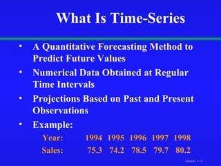
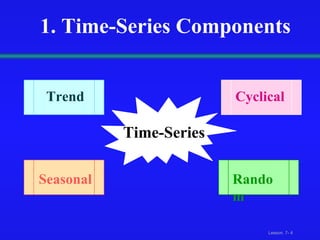
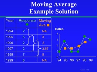
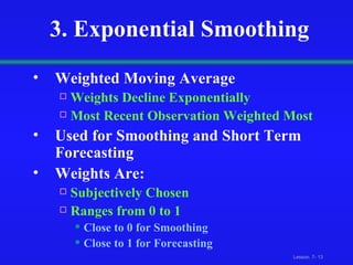
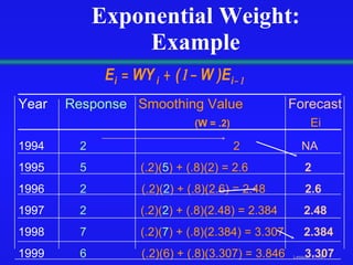
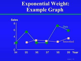
Statistics  for Management  Time-Series Analysis
Lesson Topics Component Factors of the Time-Series Model Smoothing of Data Series Moving Averages Exponential Smoothing Least Square Trend Fitting and Forecasting Linear, Quadratic and Exponential Models Autoregressive Models Choosing Appropriate Models Monthly or Quarterly Data
What Is Time-Series  A Quantitative Forecasting Method to Predict Future Values  Numerical Data Obtained at Regular Time Intervals Projections Based on Past and Present Observations Example: Year: 1994 1995 1996 1997 1998 Sales:  75.3  74.2  78.5  79.7  80.2
1. Time-Series Components Time-Series Cyclical Random Trend Seasonal
Trend Component Overall Upward or Downward Movement Data Taken Over a Period of Years Sales Time  Upward trend
Cyclical Component Upward or Downward Swings May Vary in Length Usually Lasts 2 - 10 Years Sales Time  Cycle
Seasonal Component Upward or Downward Swings Regular Patterns Observed Within 1 Year Sales Time (Monthly or Quarterly)  Winter
Random or Irregular Component Erratic, Nonsystematic, Random, ‘Residual’ Fluctuations Due to Random Variations of  Nature Accidents Short Duration and Non-repeating
Multiplicative  Time-Series Model Used Primarily for Forecasting Observed Value in Time Series is the product  of Components  For Annual Data: For Quarterly or Monthly Data: T i   = Trend C i   = Cyclical I i   = Irregular S i   = Seasonal
2. Moving Averages Used for Smoothing Series of Arithmetic Means Over Time Result Dependent Upon Choice of  L , Length of Period for Computing Means For Annual Time-Series,  L  Should be Odd  Example: 3-year Moving Average  First Average: Second Average:
Moving Average Example Year  Units   Moving   Ave 1994   2  NA 1995   5   3  1996   2   3 1997   2   3.67 1998   7  5 1999   6  NA John is a building contractor with a record of a total of 24 single family homes constructed over a 6 year period.  Provide John with a Moving Average Graph.
Moving Average Example Solution Year   Response  Moving   Ave 1994   2   NA 1995   5   3  1996   2   3 1997   2   3.67 1998   7   5 1999   6   NA 94  95  96  97  98  99 8 6 4 2 0 Sales
3. Exponential Smoothing Weighted Moving Average Weights Decline Exponentially Most Recent Observation Weighted Most Used for Smoothing and Short Term Forecasting Weights Are: Subjectively Chosen Ranges from 0 to 1 Close to 0 for Smoothing Close to 1 for Forecasting
Exponential Weight: Example Year   Response  Smoothing Value   Forecast (W = .2)   Ei 1994   2     2   NA 1995   5   (.2)( 5 ) + (.8)(2) = 2.6   2 1996   2   (.2)( 2 ) + (.8)(2.6) = 2.48  2.6 1997   2   (.2)( 2 ) + (.8)(2.48) = 2.384  2.48 1998   7   (.2)( 7 ) + (.8)(2.384) = 3.307  2.384 1999   6   (.2)(6) + (.8)(3.307) = 3.846   3.307
Exponential Weight: Example Graph 94  95  96  97  98  99 8 6 4 2 0 Sales Year Data Smoothed
4. The Linear Trend Model Year  Coded  Sales 94   0  2 95   1  5 96   2  2 97   3  2 98   4  7 99   5  6 Projected to year 2000
The Quadratic Trend Model Year  Coded  Sales 94   0  2 95   1  5 96   2  2 97   3  2 98   4  7 99   5  6
The Exponential Trend Model or Excel Output of Values in logs Year  Coded  Sales 94   0  2 95   1  5 96   2  2 97   3  2 98   4  7 99   5  6
5. Autogregressive Modeling Used for Forecasting Takes Advantage of Autocorrelation 1st order - correlation between consecutive    values 2nd order - correlation between values 2    periods apart Autoregressive Model for  pth  order: Random Error
Autoregressive Model: Example The Office Concept Corp. has acquired a number of office units (in thousands of square feet) over the last 8 years. Develop the 2nd order Autoregressive models. Year  Units   92   4 93   3 94  2   95  3  96   2  97   2  98   4 99   6
Autoregressive Model: Example Solution Year   Y i   Y i-1   Y i-2 92   4   ---  --- 93   3   4  --- 94  2   3  4 95  3   2  3 96  2  3   2 97   2  2  3 98   4  2  2 99   6  4  2 Develop the 2nd order  table run a regression model
Autoregressive Model Example: Forecasting Use the 2nd order model to forecast number of units for 2000:
Autoregressive Modeling Steps 1. Choose  p :  Note that df = n -  2p  - 1 2. Form  a series of “lag predictor” variables Y i-1  ,  Y i-2   , …  Y i-p 3. Use SPSS to run regression model using all  p  variables  4. Test significance of  A p If null hypothesis rejected, this model is selected If null hypothesis not rejected, decrease  p  by 1 and repeat
6. Selecting A Forecasting Model Perform A Residual Analysis Look for pattern or direction  Measure Sum Square Errors - SSE (residual errors) Measure Residual Errors Using MAD Use Simplest Model Principle of Parsimony
Measuring Errors Sum Square Error ( SSE ) Mean Absolute Deviation ( MAD )
Principal of Parsimony Suppose 2 or more models provide good fit for data Select the Simplest Model Simplest model types: least-squares linear least-square quadratic 1st order autoregressive More complex types: 2nd and 3rd order autoregressive least-squares exponential
Lesson Summary Discussed Component Factors of the Time-Series Model Performed Smoothing of Data Series Moving Averages Exponential Smoothing Described Least Square Trend Fitting and Forecasting -  Linear, Quadratic and Exponential Models Addressed Autoregressive Models Described Procedure for Choosing Appropriate Models Discussed Seasonal Data (use of dummy variables)

Lesson08_static11

  • 1.
    Statistics forManagement Time-Series Analysis
  • 2.
    Lesson Topics ComponentFactors of the Time-Series Model Smoothing of Data Series Moving Averages Exponential Smoothing Least Square Trend Fitting and Forecasting Linear, Quadratic and Exponential Models Autoregressive Models Choosing Appropriate Models Monthly or Quarterly Data
  • 3.
    What Is Time-Series A Quantitative Forecasting Method to Predict Future Values Numerical Data Obtained at Regular Time Intervals Projections Based on Past and Present Observations Example: Year: 1994 1995 1996 1997 1998 Sales: 75.3 74.2 78.5 79.7 80.2
  • 4.
    1. Time-Series ComponentsTime-Series Cyclical Random Trend Seasonal
  • 5.
    Trend Component OverallUpward or Downward Movement Data Taken Over a Period of Years Sales Time Upward trend
  • 6.
    Cyclical Component Upwardor Downward Swings May Vary in Length Usually Lasts 2 - 10 Years Sales Time Cycle
  • 7.
    Seasonal Component Upwardor Downward Swings Regular Patterns Observed Within 1 Year Sales Time (Monthly or Quarterly) Winter
  • 8.
    Random or IrregularComponent Erratic, Nonsystematic, Random, ‘Residual’ Fluctuations Due to Random Variations of Nature Accidents Short Duration and Non-repeating
  • 9.
    Multiplicative Time-SeriesModel Used Primarily for Forecasting Observed Value in Time Series is the product of Components For Annual Data: For Quarterly or Monthly Data: T i = Trend C i = Cyclical I i = Irregular S i = Seasonal
  • 10.
    2. Moving AveragesUsed for Smoothing Series of Arithmetic Means Over Time Result Dependent Upon Choice of L , Length of Period for Computing Means For Annual Time-Series, L Should be Odd Example: 3-year Moving Average First Average: Second Average:
  • 11.
    Moving Average ExampleYear Units Moving Ave 1994 2 NA 1995 5 3 1996 2 3 1997 2 3.67 1998 7 5 1999 6 NA John is a building contractor with a record of a total of 24 single family homes constructed over a 6 year period. Provide John with a Moving Average Graph.
  • 12.
    Moving Average ExampleSolution Year Response Moving Ave 1994 2 NA 1995 5 3 1996 2 3 1997 2 3.67 1998 7 5 1999 6 NA 94 95 96 97 98 99 8 6 4 2 0 Sales
  • 13.
    3. Exponential SmoothingWeighted Moving Average Weights Decline Exponentially Most Recent Observation Weighted Most Used for Smoothing and Short Term Forecasting Weights Are: Subjectively Chosen Ranges from 0 to 1 Close to 0 for Smoothing Close to 1 for Forecasting
  • 14.
    Exponential Weight: ExampleYear Response Smoothing Value Forecast (W = .2) Ei 1994 2 2 NA 1995 5 (.2)( 5 ) + (.8)(2) = 2.6 2 1996 2 (.2)( 2 ) + (.8)(2.6) = 2.48 2.6 1997 2 (.2)( 2 ) + (.8)(2.48) = 2.384 2.48 1998 7 (.2)( 7 ) + (.8)(2.384) = 3.307 2.384 1999 6 (.2)(6) + (.8)(3.307) = 3.846 3.307
  • 15.
    Exponential Weight: ExampleGraph 94 95 96 97 98 99 8 6 4 2 0 Sales Year Data Smoothed
  • 16.
    4. The LinearTrend Model Year Coded Sales 94 0 2 95 1 5 96 2 2 97 3 2 98 4 7 99 5 6 Projected to year 2000
  • 17.
    The Quadratic TrendModel Year Coded Sales 94 0 2 95 1 5 96 2 2 97 3 2 98 4 7 99 5 6
  • 18.
    The Exponential TrendModel or Excel Output of Values in logs Year Coded Sales 94 0 2 95 1 5 96 2 2 97 3 2 98 4 7 99 5 6
  • 19.
    5. Autogregressive ModelingUsed for Forecasting Takes Advantage of Autocorrelation 1st order - correlation between consecutive values 2nd order - correlation between values 2 periods apart Autoregressive Model for pth order: Random Error
  • 20.
    Autoregressive Model: ExampleThe Office Concept Corp. has acquired a number of office units (in thousands of square feet) over the last 8 years. Develop the 2nd order Autoregressive models. Year Units 92 4 93 3 94 2 95 3 96 2 97 2 98 4 99 6
  • 21.
    Autoregressive Model: ExampleSolution Year Y i Y i-1 Y i-2 92 4 --- --- 93 3 4 --- 94 2 3 4 95 3 2 3 96 2 3 2 97 2 2 3 98 4 2 2 99 6 4 2 Develop the 2nd order table run a regression model
  • 22.
    Autoregressive Model Example:Forecasting Use the 2nd order model to forecast number of units for 2000:
  • 23.
    Autoregressive Modeling Steps1. Choose p : Note that df = n - 2p - 1 2. Form a series of “lag predictor” variables Y i-1 , Y i-2 , … Y i-p 3. Use SPSS to run regression model using all p variables 4. Test significance of A p If null hypothesis rejected, this model is selected If null hypothesis not rejected, decrease p by 1 and repeat
  • 24.
    6. Selecting AForecasting Model Perform A Residual Analysis Look for pattern or direction Measure Sum Square Errors - SSE (residual errors) Measure Residual Errors Using MAD Use Simplest Model Principle of Parsimony
  • 25.
    Measuring Errors SumSquare Error ( SSE ) Mean Absolute Deviation ( MAD )
  • 26.
    Principal of ParsimonySuppose 2 or more models provide good fit for data Select the Simplest Model Simplest model types: least-squares linear least-square quadratic 1st order autoregressive More complex types: 2nd and 3rd order autoregressive least-squares exponential
  • 27.
    Lesson Summary DiscussedComponent Factors of the Time-Series Model Performed Smoothing of Data Series Moving Averages Exponential Smoothing Described Least Square Trend Fitting and Forecasting - Linear, Quadratic and Exponential Models Addressed Autoregressive Models Described Procedure for Choosing Appropriate Models Discussed Seasonal Data (use of dummy variables)