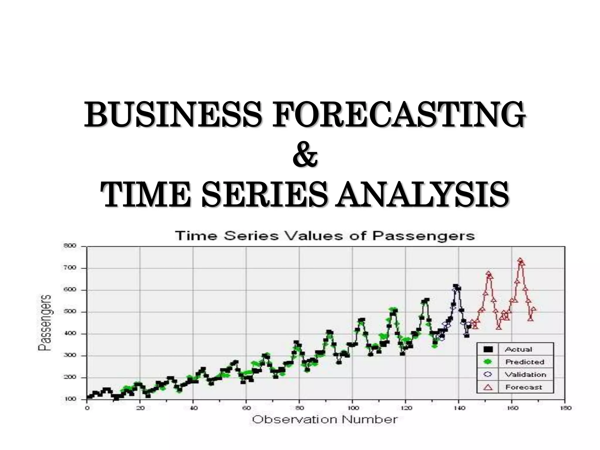
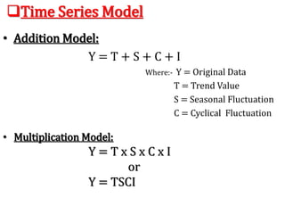
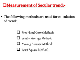
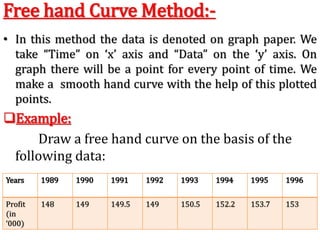
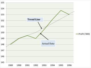
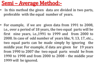
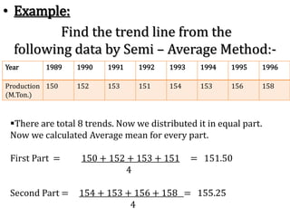
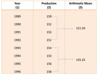
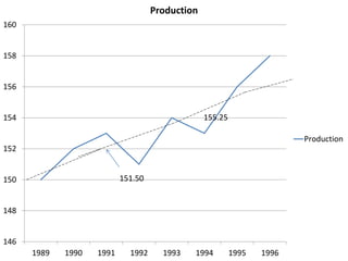
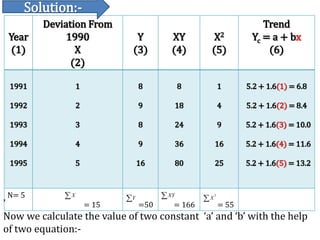
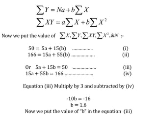
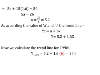
BUSINESS FORECASTING
&
TIME SERIES ANALYSIS
What is forecasting
• Forecasting is the process of making
predictions of the future based on past and
present data and most commonly by analysis
of trends.
What is business forecasting.
BUSINESS FORECASTING is an estimate or
prediction of future developments in
business such as sales, expenditures, and
profits.
Steps in forecasting
• Understanding why changes in the past have
occurred.
• Determining which phases of business activity
must be measured.
• Selecting and compiling data to be used as
measuring devices.
• Analysis of data.
Methods of forecasting
• Historical analogy method
• Field surveys and opinion method
• Business barometers
• Extrapolation
• Regression analysis
• Econometric models
• Lead leg analysis
• Exponential smoothing
• Input output analysis
• Time series analysis
TIME SERIES ANALYSIS:
Introduction:
We know that planning about future is very necessary for the
every business firm, every govt. institute, every individual and for
every country. Every family is also doing planning for his income
expenditure. As like every business is doing planning for
possibilities of its financial resources & sales and for maximization
its profit.
Definition: “A time series is a set of observation taken at
specified times, usually at equal intervals”.
“A time series may be defined as a collection of reading belonging to
different time periods of some economic or composite variables”.
By –Ya-Lun-Chau
 Time series establish relation between “cause” & “Effects”.
 One variable is “Time” which is independent variable & and the
second is “Data” which is the dependent variable.
We explain it from the following example:
• From example 1 it is clear that the sale of milk packets is decrease
from Monday to Friday then again its start to increase.
• Same thing in example 2 the population is continuously increase.
Day No. of Packets of milk sold
Monday 90
Tuesday 88
Wednesday 85
Thursday 75
Friday 72
Saturday 90
Sunday 102
Year Population (in Million)
1921 251
1931 279
1941 319
1951 361
1961 439
1971 548
1981 685
Importance of Time Series Analysis:-
As the basis of Time series Analysis businessman can
predict about the changes in economy. There are
following points which clear about the its importance:
1. Profit of experience.
2. Safety from future
3. Utility Studies
4. Sales Forecasting 5. Budgetary Analysis
6. Stock Market Analysis 7. Yield Projections
8. Process and Quality Control
9. Inventory Studies
10. Economic Forecasting
11. Risk Analysis & Evaluation of changes.
12. Census Analysis
Components of Time Series:-
The change which are being in time series, They are
effected by Economic, Social, Natural, Industrial &
Political Reasons. These reasons are called components
of Time Series.
 Secular trend :-
 Seasonal variation :-
 Cyclical variation :-
 Irregular variation :-
Secular trend:
The increase or decrease in the movements of
a time series is called Secular trend.
A time series data may show upward trend or downward trend
for a period of years and this may be due to factors like:
 increase in population,
change in technological progress ,
large scale shift in consumers demands,
For example,
• population increases over a period of time,price increases over
a period of years,production of goods on the capital market of
the country increases over a period of years.These are the
examples of upward trend.
• The sales of a commodity may decrease over a period of time
because of better products coming to the market.This is an
example of declining trend or downward.
• Seasonal variation:
• Seasonal variation are short-term fluctuation in a
time series which occur periodically in a year.
This continues to repeat year after year.
– The major factors that are weather conditions and
customs of people.
– More woolen clothes are sold in winter than in the
season of summer .
– each year more ice creams are sold in summer and
very little in Winter season.
– The sales in the departmental stores are more during
festive seasons that in the normal days.
Cyclical Variations:
Cyclical variations are recurrent upward or downward
movements in a time series but the period of cycle is
greater than a year. Also these variations are not regular
as seasonal variation.
A business cycle showing these oscillatory movements has to
pass through four phases-prosperity, recession, depression
and recovery. In a business, these four phases are
completed by passing one to another in this order.
•
• Irregular variation:
Irregular variations are fluctuations in time series that are
short in duration, erratic in nature and follow no
regularity in the occurrence pattern. These variations
are also referred to as residual variations since by
definition they represent what is left out in a time series
after trend ,cyclical and seasonal variations. Irregular
fluctuations results due to the occurrence of unforeseen
events like :
• Floods,
• Earthquakes,
• Wars,
• Famines
Time Series Model
• Addition Model:
Y = T + S + C + I
Where:- Y = Original Data
T = Trend Value
S = Seasonal Fluctuation
C = Cyclical Fluctuation
I =
I = Irregular
Fluctuation
• Multiplication Model:
Y = T x S x C x I
or
Y = TSCI
Measurement of Secular trend:-
• The following methods are used for calculation
of trend:
 Free Hand Curve Method:
 Semi – Average Method:
 Moving Average Method:
 Least Square Method:
Free hand Curve Method:-
• In this method the data is denoted on graph paper. We
take “Time” on ‘x’ axis and “Data” on the ‘y’ axis. On
graph there will be a point for every point of time. We
make a smooth hand curve with the help of this plotted
points.
Example:
Draw a free hand curve on the basis of the
following data:
Years 1989 1990 1991 1992 1993 1994 1995 1996
Profit
(in
‘000)
148 149 149.5 149 150.5 152.2 153.7 153
145
146
147
148
149
150
151
152
153
154
155
1989 1990 1991 1992 1993 1994 1995 1996
Profit ('000)
Trend Line
Actual Data
Semi – Average Method:-
• In this method the given data are divided in two parts,
preferable with the equal number of years.
• For example, if we are given data from 1991 to 2008,
i.e., over a period of 18 years, the two equal parts will be
first nine years, i.e.,1991 to 1999 and from 2000 to
2008. In case of odd number of years like, 9, 13, 17, etc..,
two equal parts can be made simply by ignoring the
middle year. For example, if data are given for 19 years
from 1990 to 2007 the two equal parts would be from
1990 to 1998 and from 2000 to 2008 - the middle year
1999 will be ignored.
• Example:
Find the trend line from the
following data by Semi – Average Method:-
Year 1989 1990 1991 1992 1993 1994 1995 1996
Production
(M.Ton.)
150 152 153 151 154 153 156 158
There are total 8 trends. Now we distributed it in equal part.
Now we calculated Average mean for every part.
First Part = 150 + 152 + 153 + 151 = 151.50
4
Second Part = 154 + 153 + 156 + 158 = 155.25
4
Year
(1)
Production
(2)
Arithmetic Mean
(3)
1989
1990
1991
1992
1993
1994
1995
1996
150
152
153
151
154
153
156
158
151.50
155.25
146
148
150
152
154
156
158
160
1989 1990 1991 1992 1993 1994 1995 1996
Production
Production
151.50
155.25
Moving Average Method:-
• It is one of the most popular method for calculating Long Term
Trend. This method is also used for ‘Seasonal fluctuation’, ‘cyclical
fluctuation’ & ‘irregular fluctuation’. In this method we calculate
the ‘Moving Average for certain years.
• For example: If we calculating ‘Three year’s Moving Average’ then
according to this method:
=(1)+(2)+(3) , (2)+(3)+(4) , (3)+(4)+(5), ……………..
3 3 3
Where (1),(2),(3),………. are the various years of time series.
Example: Find out the five year’s moving Average:
Year 1982 1983 1984 1985 1986 1987 1988 1989 1990 1991 1992 1993 1994 1995 1996
Price 20 25 33 33 27 35 40 43 35 32 37 48 50 37 45
Year
(1)
Price of
sugar (Rs.)
(2)
Five year’s moving
Total
(3)
Five year’s moving
Average (Col 3/5)
(4)
1982
1983
1984
1985
1986
1987
1988
1989
1990
1991
1992
1993
1994
1995
1996
20
25
33
30
27
35
40
43
35
32
37
48
50
37
45
-
-
135
150
165
175
180
185
187
195
202
204
217
-
-
-
-
27
30
33
35
36
27
37.4
39
40.4
40.8
43.4
-
-
• This method is most widely in practice. When this method is
applied, a trend line is fitted to data in such a manner that
the following two conditions are satisfied:-
 The sum of deviations of the actual values of y and computed
values of y is zero.
 i.e., the sum of the squares of the deviation of the actual and
computed values is least from this line. That is why method is
called the method of least squares. The line obtained by this
method is known as the line of `best fit`.
is least
Least Square Method:-
  0 cYY
 2
  cYY
The Method of least square can be used either to fit a straight line
trend or a parabolic trend.
The straight line trend is represented by the equation:-
= Yc = a + bx
Where, Y = Trend value to be computed
X = Unit of time (Independent Variable)
a = Constant to be Calculated
b = Constant to be calculated
Example:-
Draw a straight line trend and estimate trend value for 1996:
Year 1991 1992 1993 1994 1995
Production 8 9 8 9 16
Year
(1)
Deviation From
1990
X
(2)
Y
(3)
XY
(4)
X2
(5)
Trend
Yc = a + bx
(6)
1991
1992
1993
1994
1995
1
2
3
4
5
8
9
8
9
16
8
18
24
36
80
1
4
9
16
25
5.2 + 1.6(1) = 6.8
5.2 + 1.6(2) = 8.4
5.2 + 1.6(3) = 10.0
5.2 + 1.6(4) = 11.6
5.2 + 1.6(5) = 13.2
N= 5
= 15 =50 = 166 = 55
X
Y XY 2
X
’
Now we calculate the value of two constant ‘a’ and ‘b’ with the help
of two equation:-
Solution:-
  
 


2
XbXaXY
XbNaY
Now we put the value of :-
50 = 5a + 15(b) ……………. (i)
166 = 15a + 55(b) ……………… (ii)
Or 5a + 15b = 50 ……………… (iii)
15a + 55b = 166 …………………. (iv)
Equation (iii) Multiply by 3 and subtracted by (iv)
-10b = -16
b = 1.6
Now we put the value of “b” in the equation (iii)
    NXXYYX ,&,,, 2
= 5a + 15(1.6) = 50
5a = 26
a = = 5.2
As according the value of ‘a’ and ‘b’ the trend line:-
Yc = a + bx
Y= 5.2 + 1.6X
Now we calculate the trend line for 1996:-
Y1996 = 5.2 + 1.6 (6) = 14.8
5
26
m

Business forecasting and timeseries analysis phpapp02

  • 1.
  • 2.
    What is forecasting •Forecasting is the process of making predictions of the future based on past and present data and most commonly by analysis of trends. What is business forecasting. BUSINESS FORECASTING is an estimate or prediction of future developments in business such as sales, expenditures, and profits.
  • 3.
    Steps in forecasting •Understanding why changes in the past have occurred. • Determining which phases of business activity must be measured. • Selecting and compiling data to be used as measuring devices. • Analysis of data.
  • 4.
    Methods of forecasting •Historical analogy method • Field surveys and opinion method • Business barometers • Extrapolation • Regression analysis • Econometric models • Lead leg analysis • Exponential smoothing • Input output analysis • Time series analysis
  • 5.
    TIME SERIES ANALYSIS: Introduction: Weknow that planning about future is very necessary for the every business firm, every govt. institute, every individual and for every country. Every family is also doing planning for his income expenditure. As like every business is doing planning for possibilities of its financial resources & sales and for maximization its profit. Definition: “A time series is a set of observation taken at specified times, usually at equal intervals”. “A time series may be defined as a collection of reading belonging to different time periods of some economic or composite variables”. By –Ya-Lun-Chau  Time series establish relation between “cause” & “Effects”.  One variable is “Time” which is independent variable & and the second is “Data” which is the dependent variable.
  • 6.
    We explain itfrom the following example: • From example 1 it is clear that the sale of milk packets is decrease from Monday to Friday then again its start to increase. • Same thing in example 2 the population is continuously increase. Day No. of Packets of milk sold Monday 90 Tuesday 88 Wednesday 85 Thursday 75 Friday 72 Saturday 90 Sunday 102 Year Population (in Million) 1921 251 1931 279 1941 319 1951 361 1961 439 1971 548 1981 685
  • 7.
    Importance of TimeSeries Analysis:- As the basis of Time series Analysis businessman can predict about the changes in economy. There are following points which clear about the its importance: 1. Profit of experience. 2. Safety from future 3. Utility Studies 4. Sales Forecasting 5. Budgetary Analysis 6. Stock Market Analysis 7. Yield Projections 8. Process and Quality Control 9. Inventory Studies 10. Economic Forecasting 11. Risk Analysis & Evaluation of changes. 12. Census Analysis
  • 8.
    Components of TimeSeries:- The change which are being in time series, They are effected by Economic, Social, Natural, Industrial & Political Reasons. These reasons are called components of Time Series.  Secular trend :-  Seasonal variation :-  Cyclical variation :-  Irregular variation :-
  • 9.
    Secular trend: The increaseor decrease in the movements of a time series is called Secular trend. A time series data may show upward trend or downward trend for a period of years and this may be due to factors like:  increase in population, change in technological progress , large scale shift in consumers demands, For example, • population increases over a period of time,price increases over a period of years,production of goods on the capital market of the country increases over a period of years.These are the examples of upward trend. • The sales of a commodity may decrease over a period of time because of better products coming to the market.This is an example of declining trend or downward.
  • 10.
    • Seasonal variation: •Seasonal variation are short-term fluctuation in a time series which occur periodically in a year. This continues to repeat year after year. – The major factors that are weather conditions and customs of people. – More woolen clothes are sold in winter than in the season of summer . – each year more ice creams are sold in summer and very little in Winter season. – The sales in the departmental stores are more during festive seasons that in the normal days.
  • 11.
    Cyclical Variations: Cyclical variationsare recurrent upward or downward movements in a time series but the period of cycle is greater than a year. Also these variations are not regular as seasonal variation. A business cycle showing these oscillatory movements has to pass through four phases-prosperity, recession, depression and recovery. In a business, these four phases are completed by passing one to another in this order. •
  • 12.
    • Irregular variation: Irregularvariations are fluctuations in time series that are short in duration, erratic in nature and follow no regularity in the occurrence pattern. These variations are also referred to as residual variations since by definition they represent what is left out in a time series after trend ,cyclical and seasonal variations. Irregular fluctuations results due to the occurrence of unforeseen events like : • Floods, • Earthquakes, • Wars, • Famines
  • 13.
    Time Series Model •Addition Model: Y = T + S + C + I Where:- Y = Original Data T = Trend Value S = Seasonal Fluctuation C = Cyclical Fluctuation I = I = Irregular Fluctuation • Multiplication Model: Y = T x S x C x I or Y = TSCI
  • 14.
    Measurement of Seculartrend:- • The following methods are used for calculation of trend:  Free Hand Curve Method:  Semi – Average Method:  Moving Average Method:  Least Square Method:
  • 15.
    Free hand CurveMethod:- • In this method the data is denoted on graph paper. We take “Time” on ‘x’ axis and “Data” on the ‘y’ axis. On graph there will be a point for every point of time. We make a smooth hand curve with the help of this plotted points. Example: Draw a free hand curve on the basis of the following data: Years 1989 1990 1991 1992 1993 1994 1995 1996 Profit (in ‘000) 148 149 149.5 149 150.5 152.2 153.7 153
  • 16.
    145 146 147 148 149 150 151 152 153 154 155 1989 1990 19911992 1993 1994 1995 1996 Profit ('000) Trend Line Actual Data
  • 17.
    Semi – AverageMethod:- • In this method the given data are divided in two parts, preferable with the equal number of years. • For example, if we are given data from 1991 to 2008, i.e., over a period of 18 years, the two equal parts will be first nine years, i.e.,1991 to 1999 and from 2000 to 2008. In case of odd number of years like, 9, 13, 17, etc.., two equal parts can be made simply by ignoring the middle year. For example, if data are given for 19 years from 1990 to 2007 the two equal parts would be from 1990 to 1998 and from 2000 to 2008 - the middle year 1999 will be ignored.
  • 18.
    • Example: Find thetrend line from the following data by Semi – Average Method:- Year 1989 1990 1991 1992 1993 1994 1995 1996 Production (M.Ton.) 150 152 153 151 154 153 156 158 There are total 8 trends. Now we distributed it in equal part. Now we calculated Average mean for every part. First Part = 150 + 152 + 153 + 151 = 151.50 4 Second Part = 154 + 153 + 156 + 158 = 155.25 4
  • 19.
  • 20.
    146 148 150 152 154 156 158 160 1989 1990 19911992 1993 1994 1995 1996 Production Production 151.50 155.25
  • 21.
    Moving Average Method:- •It is one of the most popular method for calculating Long Term Trend. This method is also used for ‘Seasonal fluctuation’, ‘cyclical fluctuation’ & ‘irregular fluctuation’. In this method we calculate the ‘Moving Average for certain years. • For example: If we calculating ‘Three year’s Moving Average’ then according to this method: =(1)+(2)+(3) , (2)+(3)+(4) , (3)+(4)+(5), …………….. 3 3 3 Where (1),(2),(3),………. are the various years of time series. Example: Find out the five year’s moving Average: Year 1982 1983 1984 1985 1986 1987 1988 1989 1990 1991 1992 1993 1994 1995 1996 Price 20 25 33 33 27 35 40 43 35 32 37 48 50 37 45
  • 22.
    Year (1) Price of sugar (Rs.) (2) Fiveyear’s moving Total (3) Five year’s moving Average (Col 3/5) (4) 1982 1983 1984 1985 1986 1987 1988 1989 1990 1991 1992 1993 1994 1995 1996 20 25 33 30 27 35 40 43 35 32 37 48 50 37 45 - - 135 150 165 175 180 185 187 195 202 204 217 - - - - 27 30 33 35 36 27 37.4 39 40.4 40.8 43.4 - -
  • 23.
    • This methodis most widely in practice. When this method is applied, a trend line is fitted to data in such a manner that the following two conditions are satisfied:-  The sum of deviations of the actual values of y and computed values of y is zero.  i.e., the sum of the squares of the deviation of the actual and computed values is least from this line. That is why method is called the method of least squares. The line obtained by this method is known as the line of `best fit`. is least Least Square Method:-   0 cYY  2   cYY
  • 24.
    The Method ofleast square can be used either to fit a straight line trend or a parabolic trend. The straight line trend is represented by the equation:- = Yc = a + bx Where, Y = Trend value to be computed X = Unit of time (Independent Variable) a = Constant to be Calculated b = Constant to be calculated Example:- Draw a straight line trend and estimate trend value for 1996: Year 1991 1992 1993 1994 1995 Production 8 9 8 9 16
  • 25.
    Year (1) Deviation From 1990 X (2) Y (3) XY (4) X2 (5) Trend Yc =a + bx (6) 1991 1992 1993 1994 1995 1 2 3 4 5 8 9 8 9 16 8 18 24 36 80 1 4 9 16 25 5.2 + 1.6(1) = 6.8 5.2 + 1.6(2) = 8.4 5.2 + 1.6(3) = 10.0 5.2 + 1.6(4) = 11.6 5.2 + 1.6(5) = 13.2 N= 5 = 15 =50 = 166 = 55 X Y XY 2 X ’ Now we calculate the value of two constant ‘a’ and ‘b’ with the help of two equation:- Solution:-
  • 26.
          2 XbXaXY XbNaY Now we put the value of :- 50 = 5a + 15(b) ……………. (i) 166 = 15a + 55(b) ……………… (ii) Or 5a + 15b = 50 ……………… (iii) 15a + 55b = 166 …………………. (iv) Equation (iii) Multiply by 3 and subtracted by (iv) -10b = -16 b = 1.6 Now we put the value of “b” in the equation (iii)     NXXYYX ,&,,, 2
  • 27.
    = 5a +15(1.6) = 50 5a = 26 a = = 5.2 As according the value of ‘a’ and ‘b’ the trend line:- Yc = a + bx Y= 5.2 + 1.6X Now we calculate the trend line for 1996:- Y1996 = 5.2 + 1.6 (6) = 14.8 5 26
  • 28.

Editor's Notes