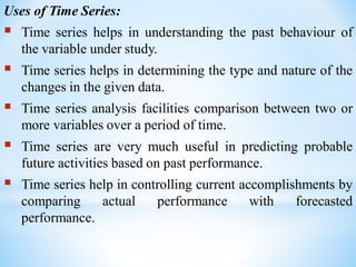
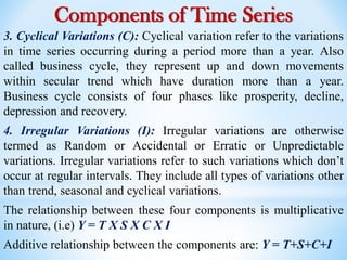
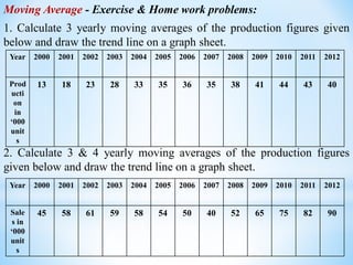
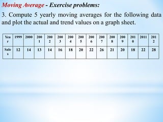
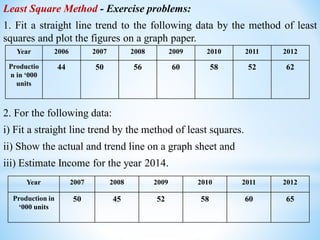
This document discusses time series analysis and its key components. It begins by defining a time series as a sequence of data points measured over successive time periods. The four main components of a time series are identified as: 1) Trend - the long-term pattern of increase or decrease, 2) Seasonal variations - repeating patterns over 12 months, 3) Cyclical variations - fluctuations lasting more than a year, and 4) Irregular variations - unpredictable fluctuations. Two common methods for measuring trends are introduced as the moving average method and least squares method. Formulas and examples are provided for calculating trend values using these techniques.

1. Mr.T.SOMASUNDARAM
ASSISTANT PROFESSOR
DEPARTMENT OF MANAGEMENT
KRISTU JAYANTI COLLEGE, BANGALORE
UNIT 4: TIME SERIES

2. UNIT 4: TIME SERIES
Meaning and Components,
Measurement of trend values
using moving average and
least square method.

3. Meaning:
In statistics, time series is a sequence of data points,
measured typically at successive time instants and spaced
at a uniform time interval.
Time series is an arrangement of data in accordance with
its time of occurrence (chronology).
Definitions:
“A Time series is a collection of magnitudes belonging
to different time periods, of some variable or composite of
variables”.
“A time series is a set of observations taken at specified
time, usually at equal intervals”.
TIME SERIES

4. Time series means a record of occurrence of a
quantitative phenomenon according to time.
Time series is defined by values Y1, Y2, Y3, …….
of a variable Y at time t1, t2, t3, ……. The
relationship between variable Y and its occurrence
is expressed as:
Y = f (t)
t represents time, which is independent variable (t1,
t2, t3, ……. tn)
Y represents value of variable, which is dependent
variable (Y1, Y2, Y3, ……………….Yn)

5. Uses of Time Series:
 Time series helps in understanding the past behaviour of
the variable under study.
 Time series helps in determining the type and nature of the
changes in the given data.
 Time series analysis facilities comparison between two or
more variables over a period of time.
 Time series are very much useful in predicting probable
future activities based on past performance.
 Time series help in controlling current accomplishments by
comparing actual performance with forecasted
performance.

6. The four components of time series are –
1. Trend Value or Secular Trend (T): Trend value or Secular
trend refers to the variations of the data over a long period of
time. The general tendency of the data to increase or decrease
during a long period of time is called trend.
(E.g.) Trend may include variations in sales, production, etc.
over 5 years.
2. Seasonal Variations (S): Seasonal variations are those
variations which occur at regular intervals and repeat during a
period of 12 months. It is due to natural causes resulting from
changes in weather and climatic conditions and human causes
like changes in customer taste, habit, etc.
(E.g.) monthly production & sales, interest payments, etc.
Components of Time Series

7. 3. Cyclical Variations (C): Cyclical variation refer to the variations
in time series occurring during a period more than a year. Also
called business cycle, they represent up and down movements
within secular trend which have duration more than a year.
Business cycle consists of four phases like prosperity, decline,
depression and recovery.
4. Irregular Variations (I): Irregular variations are otherwise
termed as Random or Accidental or Erratic or Unpredictable
variations. Irregular variations refer to such variations which don’t
occur at regular intervals. They include all types of variations other
than trend, seasonal and cyclical variations.
The relationship between these four components is multiplicative
in nature, (i.e) Y = T X S X C X I
Additive relationship between the components are: Y = T+S+C+I
Components of Time Series

8. *
Computation of Trend Values

9. *
Computation of Trend Values

10. Moving Average - Exercise & Home work problems:
1. Calculate 3 yearly moving averages of the production figures given
below and draw the trend line on a graph sheet.
2. Calculate 3 & 4 yearly moving averages of the production figures
given below and draw the trend line on a graph sheet.
Year 2000 2001 2002 2003 2004 2005 2006 2007 2008 2009 2010 2011 2012
Prod
ucti
on
in
‘000
unit
s
13 18 23 28 33 35 36 35 38 41 44 43 40
Year 2000 2001 2002 2003 2004 2005 2006 2007 2008 2009 2010 2011 2012
Sale
s in
‘000
unit
s
45 58 61 59 58 54 50 40 52 65 75 82 90

11. Moving Average - Exercise problems:
3. Compute 5 yearly moving averages for the following data
and plot the actual and trend values on a graph sheet.
Yea
r
1999 2000 200
1
200
2
200
3
200
4
200
5
200
6
200
7
200
8
200
9
201
0
2011 201
2
Sale
s
12 14 13 14 16 18 20 22 26 21 20 18 22 28

12. 2. Least Square Method:
This method is used to finding trend values based on
regression techniques.
Definition:
“Least Square method is the sum of the squares of the
individual deviations between actual values and computed
trend values will be least.”
The straight line representing trend values, we get when
plotted on a graph sheet, under the method of least squares is
known as the ‘Line of Best Fit’.
Computation of Trend Values

13. 2. Least Square Method - Formula:
Trend line equation is Yc = a + bX
where Yc – trend value, a = Y intercept when X = 0
The value ‘a’ and ‘b’ are constants in equation and it is solved
by using simultaneous equation.
To find ‘a’ and ‘b’,
∑Y = Na + b∑X
∑XY = a∑X + b∑X2
where N – total no. of time periods, X – time deviations
Y – actual values, ‘a’ and ‘b’ are constants.
Computation of Trend Values

14. Least Square Method - Exercise problems:
1. Fit a straight line trend to the following data by the method of least
squares and plot the figures on a graph paper.
2. For the following data:
i) Fit a straight line trend by the method of least squares.
ii) Show the actual and trend line on a graph sheet and
iii) Estimate Income for the year 2014.
Year 2006 2007 2008 2009 2010 2011 2012
Productio
n in ‘000
units
44 50 56 60 58 52 62
Year 2007 2008 2009 2010 2011 2012
Production in
‘000 units
50 45 52 58 60 65

15. Least Square Method - Homework problems:
1. Fit a straight line to the following data by the method of least squares.
2. Given below are the figures of demand for a commodity:
i) Fit a straight line by ‘Least squares’ method.
ii) Show the actual and trend line on a graph sheet and
iii) Estimate the demand for the year 2013.
Year 2006 2007 2008 2009 2010 2011 2012
Production in
‘000 units
100 120 136 124 118 132 140
Year 2006 2007 2008 2009 2010 2011 2012
Demand in
‘000 units
73 85 74 75 80 52 58

16. End of the Unit 4
Thank You