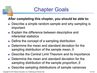
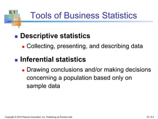
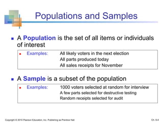
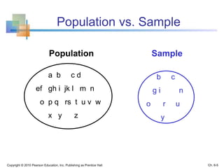
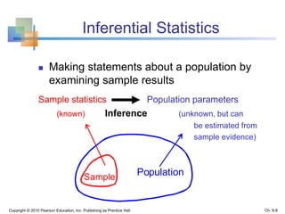
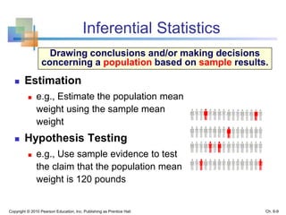
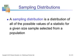
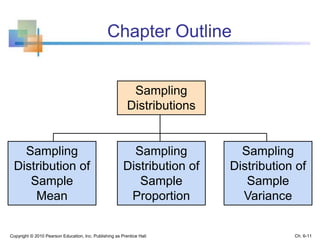
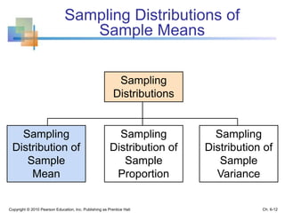
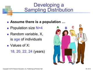
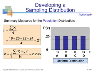
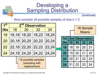
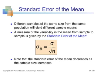
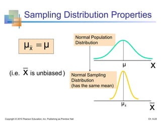
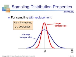
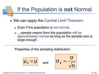
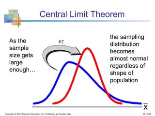
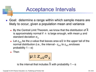
Chap06 sampling and sampling distributions

Copyright © 2010 Pearson Education, Inc. Publishing as Prentice Hall
Statistics for
Business and Economics
7th Edition
Chapter 6
Sampling and
Sampling Distributions
Ch. 6-1

Chapter Goals
After completing this chapter, you should be able to:
 Describe a simple random sample and why sampling is
important
 Explain the difference between descriptive and
inferential statistics
 Define the concept of a sampling distribution
 Determine the mean and standard deviation for the
sampling distribution of the sample mean,
 Describe the Central Limit Theorem and its importance
 Determine the mean and standard deviation for the
sampling distribution of the sample proportion,
 Describe sampling distributions of sample variances
pˆ
X
Copyright © 2010 Pearson Education, Inc. Publishing as Prentice Hall Ch. 6-2

Tools of Business Statistics
 Descriptive statistics
 Collecting, presenting, and describing data
 Inferential statistics
 Drawing conclusions and/or making decisions
concerning a population based only on
sample data
6.1

Populations and Samples
 A Population is the set of all items or individuals
of interest
 Examples: All likely voters in the next election
All parts produced today
All sales receipts for November
 A Sample is a subset of the population
 Examples: 1000 voters selected at random for interview
A few parts selected for destructive testing
Random receipts selected for audit

Population vs. Sample
a b c d
ef gh i jk l m n
o p q rs t u v w
x y z
Population Sample
b c
g i n
o r u
y
Ch. 6-5

Why Sample?
 Less time consuming than a census
 Less costly to administer than a census
 It is possible to obtain statistical results of a
sufficiently high precision based on samples.

Simple Random Samples
 Every object in the population has an equal chance of
being selected
 Objects are selected independently
 Samples can be obtained from a table of random
numbers or computer random number generators
 A simple random sample is the ideal against which
other sample methods are compared

Inferential Statistics
 Making statements about a population by
examining sample results
Sample statistics Population parameters
(known) Inference (unknown, but can
be estimated from
sample evidence)
Sample Population
Ch. 6-8

Inferential Statistics
 Estimation
 e.g., Estimate the population mean
weight using the sample mean
weight
 Hypothesis Testing
 e.g., Use sample evidence to test
the claim that the population mean
weight is 120 pounds
Drawing conclusions and/or making decisions
concerning a population based on sample results.
Ch. 6-9

Sampling Distributions
 A sampling distribution is a distribution of
all of the possible values of a statistic for
a given size sample selected from a
population
6.2

Chapter Outline
Sampling
Distributions
Sampling
Distribution of
Sample
Mean
Sampling
Distribution of
Sample
Proportion
Sampling
Distribution of
Sample
Variance
Ch. 6-11

Sampling Distributions of
Sample Means
Sampling
Distributions
Sampling
Distribution of
Sample
Mean
Sampling
Distribution of
Sample
Proportion
Sampling
Distribution of
Sample
Variance
Ch. 6-12

Developing a
Sampling Distribution
 Assume there is a population …
 Population size N=4
 Random variable, X,
is age of individuals
 Values of X:
18, 20, 22, 24 (years)
A B C D
Ch. 6-13

Developing a
.25
0
18 20 22 24
A B C D
Uniform Distribution
P(x)
x
(continued)
Summary Measures for the Population Distribution:
21
4
24222018
N
X
μ i





2.236
N
μ)(X
σ
2
i




Ch. 6-14

Now consider all possible samples of size n = 2
1st
2nd
Observation
Obs 18 20 22 24
18 18,18 18,20 18,22 18,24
20 20,18 20,20 20,22 20,24
22 22,18 22,20 22,22 22,24
24 24,18 24,20 24,22 24,24
16 possible samples
(sampling with
replacement)
1st 2nd Observation
Obs 18 20 22 24
18 18 19 20 21
20 19 20 21 22
22 20 21 22 23
24 21 22 23 24
(continued)
Developing a
16 Sample
Means
Ch. 6-15

Sampling Distribution of All Sample Means
1st 2nd Observation
Obs 18 20 22 24
18 18 19 20 21
20 19 20 21 22
22 20 21 22 23
24 21 22 23 24 18 19 20 21 22 23 24
0
.1
.2
.3
P(X)
X
Sample Means
Distribution
16 Sample Means
_
Developing a
(continued)
(no longer uniform)
_
Ch. 6-16

Summary Measures of this Sampling Distribution:
Developing a
(continued)
μ21
16
24211918
N
X
)XE( i



 
1.58
16
21)-(2421)-(1921)-(18
N
μ)X(
σ
222
2
i
X







Ch. 6-17

Comparing the Population with its
18 19 20 21 22 23 24
0
.1
.2
.3
P(X)
X18 20 22 24
A B C D
0
.1
.2
.3
Population
N = 4
P(X)
X
_
1.58σ21μ XX
2.236σ21μ 
Sample Means Distribution
n = 2
_
Ch. 6-18

Expected Value of Sample Mean
 Let X1, X2, . . . Xn represent a random sample from a
population
 The sample mean value of these observations is
defined as


n
1i
iX
n
1
X
Ch. 6-19

Standard Error of the Mean
 Different samples of the same size from the same
population will yield different sample means
 A measure of the variability in the mean from sample to
sample is given by the Standard Error of the Mean:
 Note that the standard error of the mean decreases as
the sample size increases
n
σ
σX

Ch. 6-20

If sample values are
not independent
 If the sample size n is not a small fraction of the
population size N, then individual sample members
are not distributed independently of one another
 Thus, observations are not selected independently
 A correction is made to account for this:
or
(continued)
1N
nN
n
σ
σX



1N
nN
n
σ
)XVar(
2




If the Population is Normal
 If a population is normal with mean μ and
standard deviation σ, the sampling distribution
of is also normally distributed with
and
 If the sample size n is not large relative to the population size N, then
and
X
μμX

n
σ
σX

Ch. 6-22
1N
nN
n
σ
σX


μμX


Z-value for Sampling Distribution
of the Mean
 Z-value for the sampling distribution of :
where: = sample mean
= population mean
= standard error of the mean
X
μ
X
σ
μ)X(
Z


X
Ch. 6-23
xσ

Sampling Distribution Properties
(i.e. is unbiased )
Normal Population
Distribution
Normal Sampling
Distribution
(has the same mean)
x
x
x
μμx 
μ
xμ
Ch. 6-24

Sampling Distribution Properties
 For sampling with replacement:
As n increases,
decreases
Larger
sample size
Smaller
sample size
x
(continued)
xσ
μ
Ch. 6-25

If the Population is not Normal
 We can apply the Central Limit Theorem:
 Even if the population is not normal,
 …sample means from the population will be
approximately normal as long as the sample size is
large enough.
Properties of the sampling distribution:
and
μμx 
n
σ
σx 
Ch. 6-26

Central Limit Theorem
n↑As the
sample
size gets
large
enough…
the sampling
distribution
becomes
almost normal
regardless of
shape of
population
x
Ch. 6-27

If the Population is not Normal
Population Distribution
(becomes normal as n increases)
Central Tendency
Variation
x
x
Larger
sample
size
Smaller
sample size
(continued)
Sampling distribution
properties:
μμx 
n
σ
σx 
xμ
μ
Ch. 6-28

How Large is Large Enough?
 For most distributions, n > 25 will give a
sampling distribution that is nearly normal
 For normal population distributions, the
sampling distribution of the mean is always
normally distributed

Example
 Suppose a large population has mean μ = 8
and standard deviation σ = 3. Suppose a
random sample of size n = 36 is selected.
 What is the probability that the sample mean is
between 7.8 and 8.2?

Example
Solution:
 Even if the population is not normally
distributed, the central limit theorem can be
used (n > 25)
 … so the sampling distribution of is
approximately normal
 … with mean = 8
 …and standard deviation
(continued)
x
xμ
0.5
36
3
n
σ
σx 
Ch. 6-31

Example
Solution (continued):
(continued)
0.38300.5)ZP(-0.5
36
3
8-8.2
n
σ
μ-μ
36
3
8-7.8
P8.2)μP(7.8
X
X












Z7.8 8.2 -0.5 0.5
Sampling
Distribution
Standard Normal
Distribution .1915
+.1915
Population
Distribution
?
?
?
?
????
?
???
Sample Standardize
8μ  8μX
 0μz xX
Ch. 6-32

Acceptance Intervals
 Goal: determine a range within which sample means are
likely to occur, given a population mean and variance
 By the Central Limit Theorem, we know that the distribution of X
is approximately normal if n is large enough, with mean μ and
standard deviation
 Let zα/2 be the z-value that leaves area α/2 in the upper tail of the
normal distribution (i.e., the interval - zα/2 to zα/2 encloses
probability 1 – α)
 Then
is the interval that includes X with probability 1 – α
X
σ
X/2σzμ 
Ch. 6-33

Sampling
Distributions
Sampling
Distribution of
Sample
Mean
Sampling
Distribution of
Sample
Proportion
Sampling
Distribution of
Sample
Variance
Ch. 6-34
Sample Proportions
6.3

Sample Proportions
P = the proportion of the population having
some characteristic
 Sample proportion ( ) provides an estimate
of P:
 0 ≤ ≤ 1
 has a binomial distribution, but can be approximated
by a normal distribution when nP(1 – P) > 5
sizesample
interestofsticcharacterithehavingsampletheinitemsofnumber
n
X
p ˆ
pˆ
pˆ
Ch. 6-35
pˆ

Sampling Distribution of p
 Normal approximation:
Properties:
and
(where P = population proportion)
.3
.2
.1
0
0 . 2 .4 .6 8 1
P)pE( ˆ
n
P)P(1
n
X
Varσ2
p







ˆ
^
)PP(ˆ
Pˆ
Ch. 6-36

Z-Value for Proportions
n
P)P(1
Pp
σ
Pp
Z
p 




ˆˆ
ˆ
Standardize to a Z value with the formula:
Ch. 6-37
pˆ

Example
 If the true proportion of voters who support
Proposition A is P = .4, what is the probability
that a sample of size 200 yields a sample
proportion between .40 and .45?
 i.e.: if P = .4 and n = 200, what is
P(.40 ≤ ≤ .45) ?pˆ
Ch. 6-38

Example
 if P = .4 and n = 200, what is
P(.40 ≤ ≤ .45) ?
(continued)
.03464
200
.4).4(1
n
P)P(1
σp




ˆ
1.44)ZP(0
.03464
.40.45
Z
.03464
.40.40
P.45)pP(.40






 


 ˆ
Find :
Convert to
standard
normal:
p
σˆ
Ch. 6-39
pˆ

Example
 if P = .4 and n = 200, what is
P(.40 ≤ ≤ .45) ?
Z.45 1.44
.4251
Standardize
Standardized
Normal Distribution
(continued)
Use standard normal table: P(0 ≤ Z ≤ 1.44) = .4251
.40 0pˆ
Ch. 6-40
pˆ

Sample Variance
Sampling
Distributions
Sampling
Distribution of
Sample
Mean
Sampling
Distribution of
Sample
Proportion
Sampling
Distribution of
Sample
Variance
Ch. 6-41
6.4

Sample Variance
 Let x1, x2, . . . , xn be a random sample from a
population. The sample variance is
 the square root of the sample variance is called
the sample standard deviation
 the sample variance is different for different
random samples from the same population




n
1i
2
i
2
)x(x
1n
1
s
Ch. 6-42

Sampling Distribution of
Sample Variances
 The sampling distribution of s2 has mean σ2
 If the population distribution is normal, then
 If the population distribution is normal then
has a 2 distribution with n – 1 degrees of freedom
22
σ)E(s 
1n
2σ
)Var(s
4
2


2
2
σ
1)s-(n
Ch. 6-43

The Chi-square Distribution
 The chi-square distribution is a family of distributions,
depending on degrees of freedom:
 d.f. = n – 1
 Text Table 7 contains chi-square probabilities
0 4 8 12 16 20 24 28 0 4 8 12 16 20 24 28 0 4 8 12 16 20 24 28
d.f. = 1 d.f. = 5 d.f. = 15
2 22
Ch. 6-44

Degrees of Freedom (df)
Idea: Number of observations that are free to vary
after sample mean has been calculated
Example: Suppose the mean of 3 numbers is 8.0
Let X1 = 7
Let X2 = 8
What is X3?
If the mean of these three
values is 8.0,
then X3 must be 9
(i.e., X3 is not free to vary)
Here, n = 3, so degrees of freedom = n – 1 = 3 – 1 = 2
(2 values can be any numbers, but the third is not free to vary
for a given mean)
Ch. 6-45

Chi-square Example
 A commercial freezer must hold a selected
temperature with little variation. Specifications call
for a standard deviation of no more than 4 degrees
(a variance of 16 degrees2).
 A sample of 14 freezers is to be
tested
 What is the upper limit (K) for the
sample variance such that the
probability of exceeding this limit,
given that the population standard
deviation is 4, is less than 0.05?
Ch. 6-46

Finding the Chi-square Value
 Use the the chi-square distribution with area 0.05
in the upper tail:
probability
α = .05
2
13
2
2
13
= 22.36
= 22.36 (α = .05 and 14 – 1 = 13 d.f.)
2
2
2
σ
1)s(n 
χ
Is chi-square distributed with (n – 1) = 13
degrees of freedom
Ch. 6-47

Chi-square Example
0.05
16
1)s(n
PK)P(s 2
13
2
2








 χSo:
(continued)
2
13 = 22.36 (α = .05 and 14 – 1 = 13 d.f.)
22.36
16
1)K(n

 (where n = 14)
so 27.52
1)(14
)(22.36)(16
K 


If s2 from the sample of size n = 14 is greater than 27.52, there is
strong evidence to suggest the population variance exceeds 16.
or
Ch. 6-48

Chapter Summary
 Introduced sampling distributions
 Described the sampling distribution of sample means
 For normal populations
 Using the Central Limit Theorem
 Described the sampling distribution of sample
proportions
 Introduced the chi-square distribution
 Examined sampling distributions for sample variances
 Calculated probabilities using sampling distributions

Chap06 sampling and sampling distributions

More Related Content

What's hot

Similar to Chap06 sampling and sampling distributions

More from Judianto Nugroho

Recently uploaded

Chap06 sampling and sampling distributions