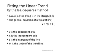
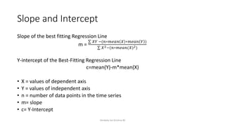
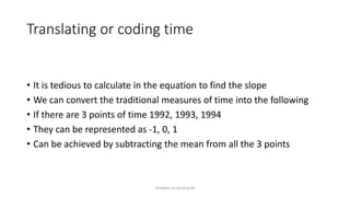
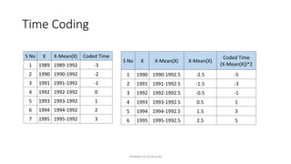
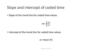
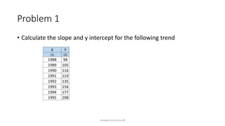
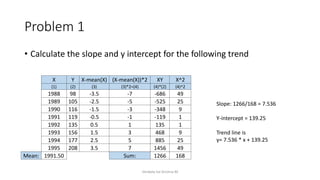
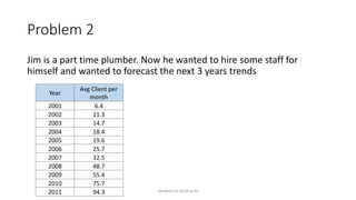
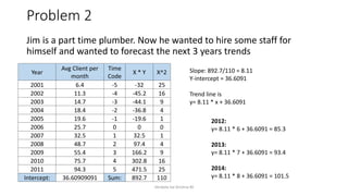
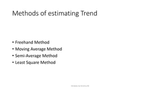
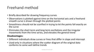
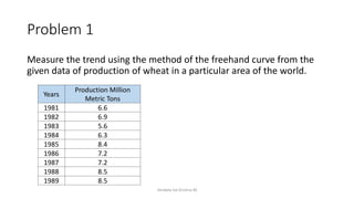
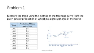
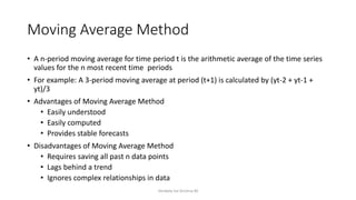
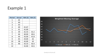
Time series and forecasting

Time Series and Forecasting
Venkata Sai Krishna M

Introduction
• Forecasting or predicting is an essential tool in any decision-making
process
• Used for Inventory management to annual sales
• Quality depends on the quantity of the past data
• Pattern is used to arrive at an estimate in the future
• This analysis helps us cope with uncertainty about the future

Variations in Time Series
4 different variation involved in time series:
1. Secular Trend
2. Cyclical Fluctuation
3. Seasonal Variation
4. Irregular Variation

Secular Trend
• The value of the variable tends to increase or decrease over a long
period
• Steady increase in cost of living recorded by the Consumer Price Index
is an example of secular trend
• In terms of long term period, complete cost of living varies a great
deal

Cyclical Trend
• Business cycle is the most common example
• Peak at sometimes and likely to slump at the other
• The cycle may extend up to 1 year to 15 to 20 years
• There is no regular pattern but will move in little unpredictable
manner

Seasonal Variation
• Involves patterns of change within a year
• They tend to have a cycle from year to year
• Substantial peak and irregular through at particular periods in a year

Irregular Variations
• Value of a variable may be completely unpredictable
• Effect of one situation ripples to the impact of any other inter related
commodity
• White Revolution and effect on Gas

Reasons for Studying Trends
• The study of secular trends allows us to describe a historical pattern
• Evaluating the eating lifecycle resulted in creation of Maggie
• Studying secular trends permits us to project past patterns, or trends,
into the future
• Growth trend of population helps predict the population projections
• In many situations, studying the secular trend of a time series allows
us to eliminate the trend component from the series
• Make in India Campaign

Fitting the Linear Trend
by the least-squares method
• Assuming the trend is in the straight line
• The general equation of a straight line:
y = mx + c
• y is the dependent axis
• X is the independent axis
• c is the intercept of the line
• m is the slope of the trend line

Slope and Intercept
Slope of the best fitting Regression Line
m =
𝑋𝑌 −(𝑛∗𝑚𝑒𝑎𝑛 𝑋 ∗𝑚𝑒𝑎𝑛 𝑌 )
𝑋2−(𝑛∗𝑚𝑒𝑎𝑛(𝑋)2)
Y-intercept of the Best-Fitting Regression Line
c=mean(Y)-m*mean(X)
• X = values of dependent axis
• Y = values of independent axis
• n = number of data points in the time series
• m= slope
• c= Y-Intercept

Translating or coding time
• It is tedious to calculate in the equation to find the slope
• We can convert the traditional measures of time into the following
• If there are 3 points of time 1992, 1993, 1994
• They can be represented as -1, 0, 1
• Can be achieved by subtracting the mean from all the 3 points

Time Coding
S No X X-Mean(X) Coded Time
1 1989 1989-1992 -3
2 1990 1990-1992 -2
3 1991 1991-1992 -1
4 1992 1992-1992 0
5 1993 1993-1992 1
6 1994 1994-1992 2
7 1995 1995-1992 3
S No X X-Mean(X) X-Mean(X)
Coded Time
(X-Mean(X))*2
1 1990 1990-1992.5 -2.5 -5
2 1991 1991-1992.5 -1.5 -3
3 1992 1992-1992.5 -0.5 -1
4 1993 1993-1992.5 0.5 1
5 1994 1994-1992.5 1.5 3
6 1995 1995-1992.5 2.5 5

Slope and intercept of coded time
• Slope of the trend line for coded time values
m=
𝑥𝑌
𝑥2
• Intercept of the trend line for coded time values
a= mean (Y)

Problem 1
• Calculate the slope and y intercept for the following trend
X Y
(1) (2)
1988 98
1989 105
1990 116
1991 119
1992 135
1993 156
1994 177
1995 208

Problem 1
• Calculate the slope and y intercept for the following trend
X Y X-mean(X) (X-mean(X))*2 XY X^2
(1) (2) (3) (3)*2=(4) (4)*(2) (4)^2
1988 98 -3.5 -7 -686 49
1989 105 -2.5 -5 -525 25
1990 116 -1.5 -3 -348 9
1991 119 -0.5 -1 -119 1
1992 135 0.5 1 135 1
1993 156 1.5 3 468 9
1994 177 2.5 5 885 25
1995 208 3.5 7 1456 49
Mean: 1991.50 Sum: 1266 168
Slope: 1266/168 = 7.536
Y-intercept = 139.25
Trend line is
y= 7.536 * x + 139.25

Problem 2
Jim is a part time plumber. Now he wanted to hire some staff for
himself and wanted to forecast the next 3 years trends
Year
Avg Client per
month
2001 6.4
2002 11.3
2003 14.7
2004 18.4
2005 19.6
2006 25.7
2007 32.5
2008 48.7
2009 55.4
2010 75.7
2011 94.3

Problem 2
Jim is a part time plumber. Now he wanted to hire some staff for
himself and wanted to forecast the next 3 years trends
Year
Avg Client per
month
Time
Code
X * Y X^2
2001 6.4 -5 -32 25
2002 11.3 -4 -45.2 16
2003 14.7 -3 -44.1 9
2004 18.4 -2 -36.8 4
2005 19.6 -1 -19.6 1
2006 25.7 0 0 0
2007 32.5 1 32.5 1
2008 48.7 2 97.4 4
2009 55.4 3 166.2 9
2010 75.7 4 302.8 16
2011 94.3 5 471.5 25
Intercept: 36.60909091 Sum: 892.7 110
Slope: 892.7/110 = 8.11
Y-intercept = 36.6091
Trend line is
y= 8.11 * x + 36.6091
2012:
y= 8.11 * 6 + 36.6091 = 85.3
2013:
y= 8.11 * 7 + 36.6091 = 93.4
2014:
y= 8.11 * 8 + 36.6091 = 101.5

Methods of estimating Trend
• Freehand Method
• Moving Average Method
• Semi-Average Method
• Least Square Method

Freehand method
• Briefly described for drawing frequency curves
• Observations is plotted against time on the horizontal axis and a freehand
smooth curve is drawn through the plotted points
• Smoothness should not be scarified in trying to let the points fall exactly on
the curve
• Eliminates the short term and long term oscillations and the irregular
movements from the time series, and elevates the general trend
Disadvantages:
• Different individuals draw curves or lines that differ in slope and intercept
• Used only in situations where the scatter diagram of the original data
conforms to some well define trends

Problem 1
Measure the trend using the method of the freehand curve from the
given data of production of wheat in a particular area of the world.
Years
Production Million
Metric Tons
1981 6.6
1982 6.9
1983 5.6
1984 6.3
1985 8.4
1986 7.2
1987 7.2
1988 8.5
1989 8.5

Moving Average Method
• A n-period moving average for time period t is the arithmetic average of the time series
values for the n most recent time periods
• For example: A 3-period moving average at period (t+1) is calculated by (yt-2 + yt-1 +
yt)/3
• Advantages of Moving Average Method
• Easily understood
• Easily computed
• Provides stable forecasts
• Disadvantages of Moving Average Method
• Requires saving all past n data points
• Lags behind a trend
• Ignores complex relationships in data

Example 1
Period Actual MA (3) MA (5)
1 42
2 40
3 43
4 40 41.67
5 41 41.00
6 39 41.33 41.2
7 46 40.00 40.6
8 44 42.00 41.8
9 45 43.00 42
10 38 45.00 43
11 40 42.33 42.4
12 41.00 42.6
34
36
38
40
42
44
46
48
1 2 3 4 5 6 7 8 9 10 11 12
Weighted Moving Average
Actual MA (3) MA (5)

Semi Average Method
• This method is as simple and relatively objective as the free hand
method
• Data is divided in two equal halves and the arithmetic mean is
calculated
• If the number of observations is even the division into halves
• If the number of observations is odd, then the middle most item is
dropped

Advantages and Disadvantages of the Semi-
Averages Method
• Advantages
• This method is very simple and easy to understand, and also it does
not require many calculations.
• Disadvantages
• For non-linear trends this method is not applicable.
• averages are affected by extreme values
• extreme value should either be omitted or this method should not be
applied

Example 1

Example 1 Solutions

Example 1 Solution
• Trend of 1 year is called the
slope = m = 3.656
• Trend of 1st year in the
series is the y –intercept = c
= 25.008
• Then the trend line is
y= 3.656x + 25.008

Time series and forecasting

More Related Content

What's hot

Similar to Time series and forecasting

Recently uploaded

Time series and forecasting