Download as PDF, PPTX


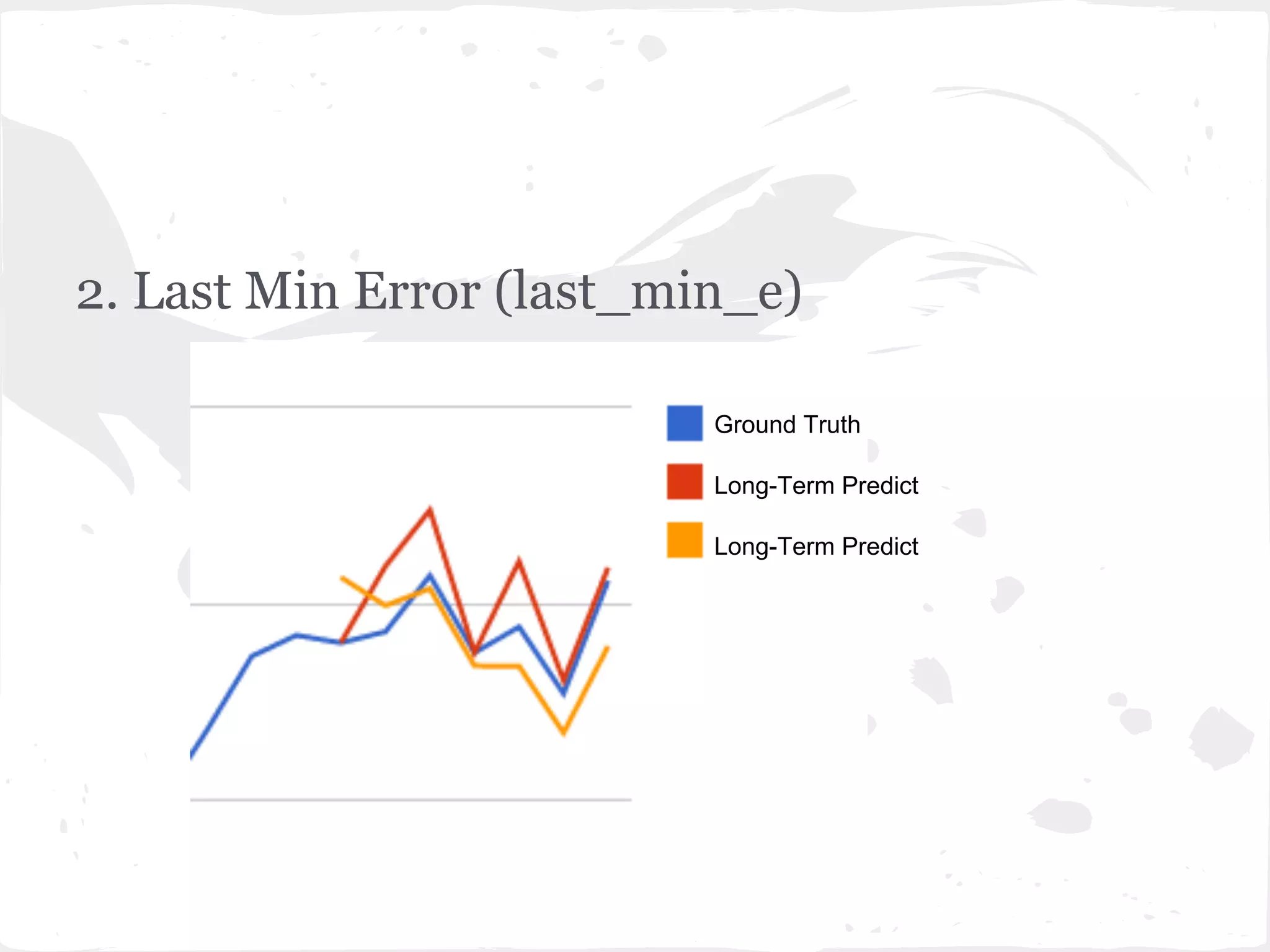
![2. Last Min Error (last_min_e)
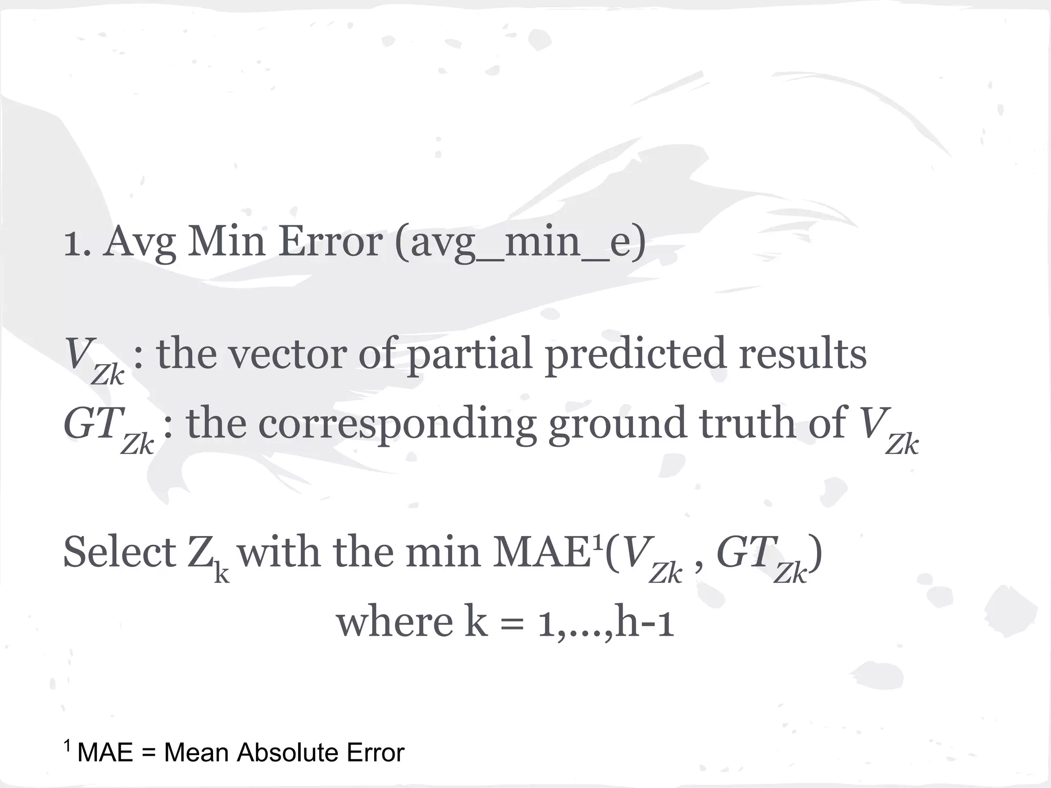
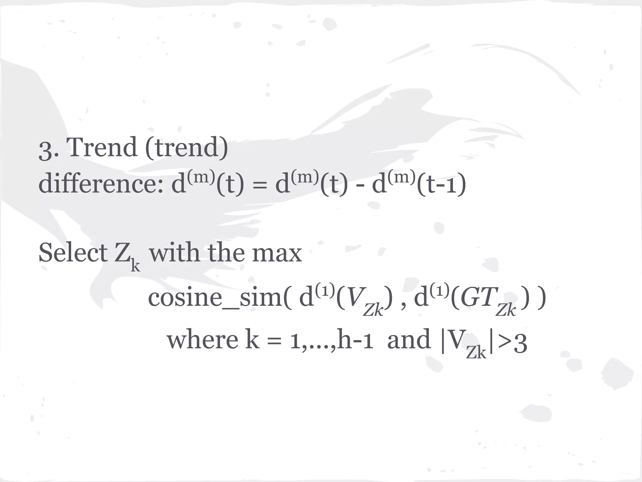
Select Zk
with the min MAE( VZk
[1] , GTZk
[1] )
where k = 1,...,h-1](https://image.slidesharecdn.com/slideprintfororal-150808091422-lva1-app6891/75/A-General-Framework-for-Enhancing-Prediction-Performance-on-Time-Series-Data-60-2048.jpg)

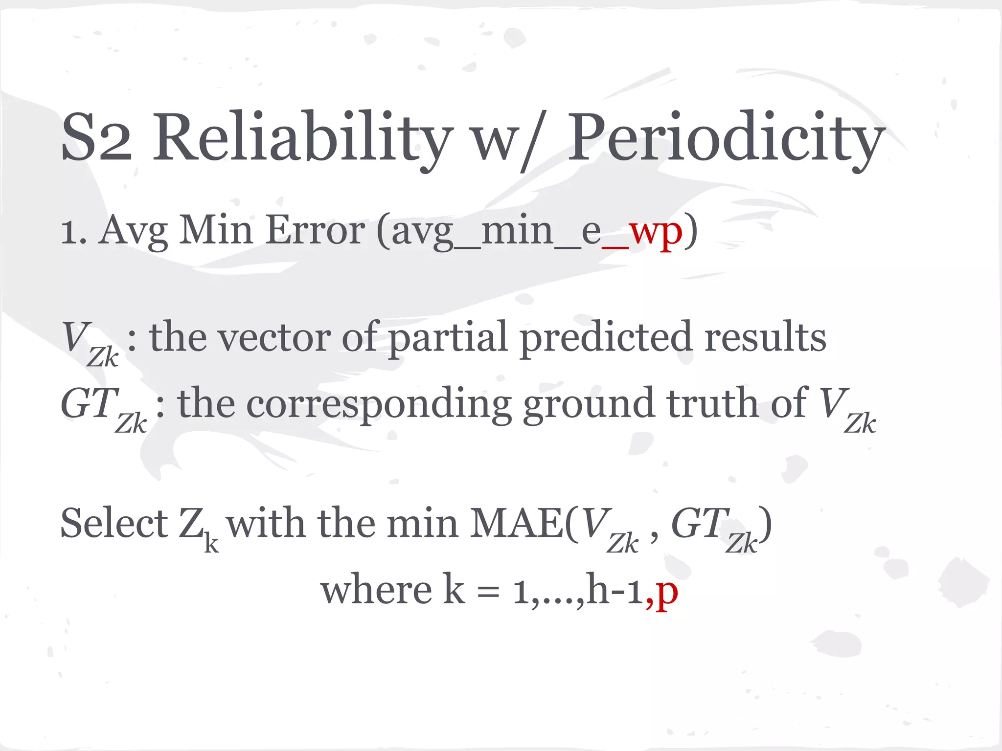
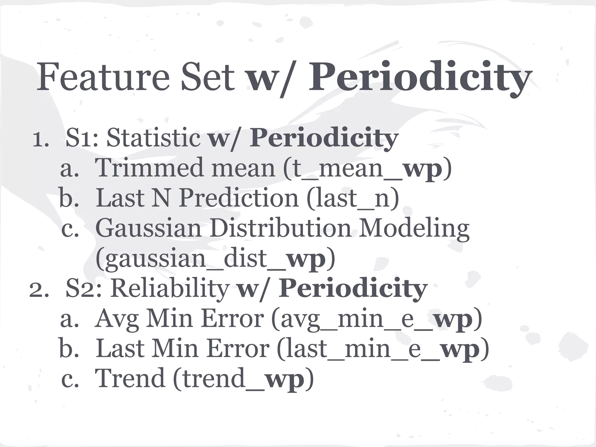
![2. Last Min Error (last_min_e_wp)
Select Zk
with the min MAE( VZk
[1] , GTZk
[1] )
where k = 1,...,h-1,p](https://image.slidesharecdn.com/slideprintfororal-150808091422-lva1-app6891/75/A-General-Framework-for-Enhancing-Prediction-Performance-on-Time-Series-Data-70-2048.jpg)
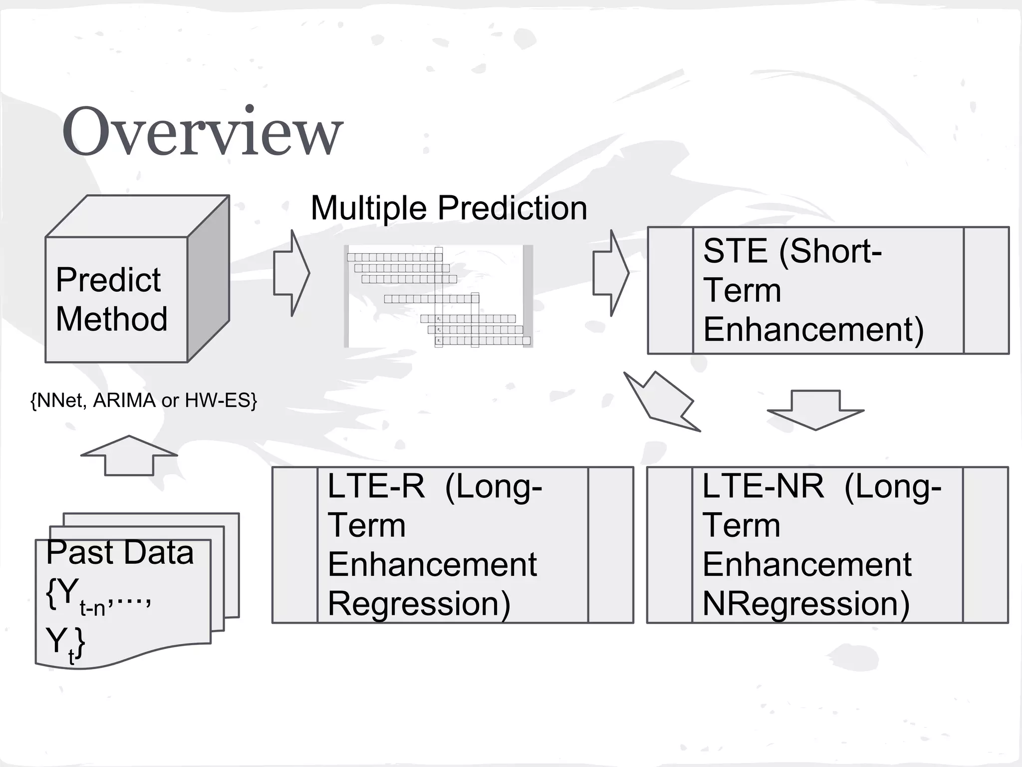
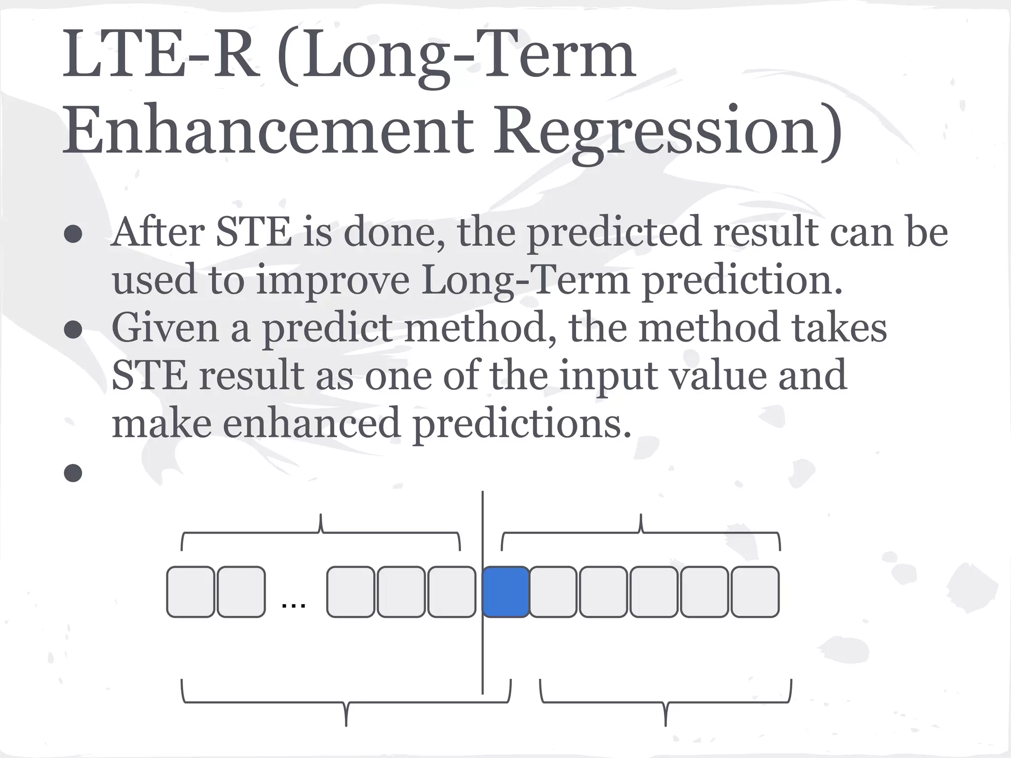
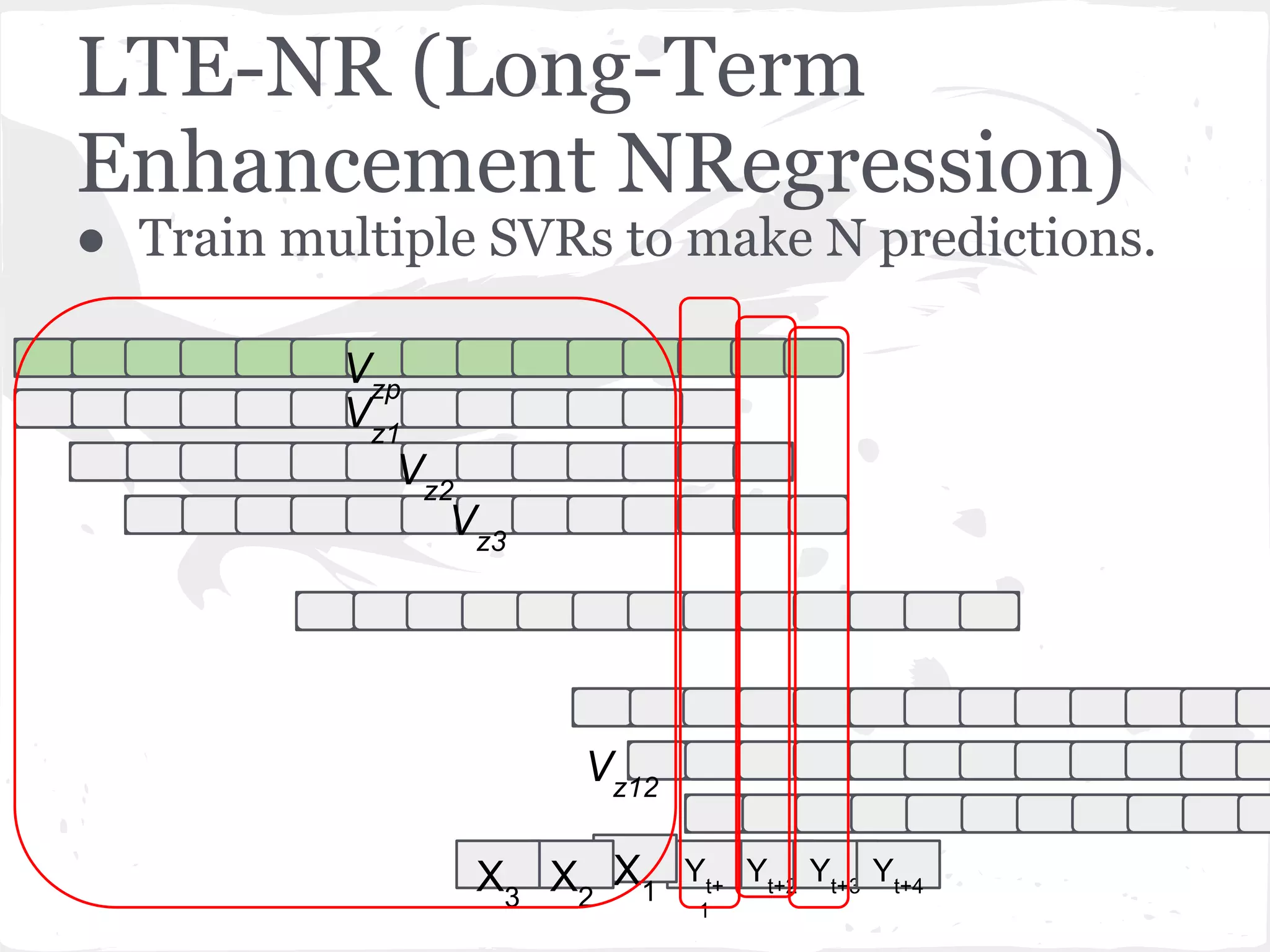


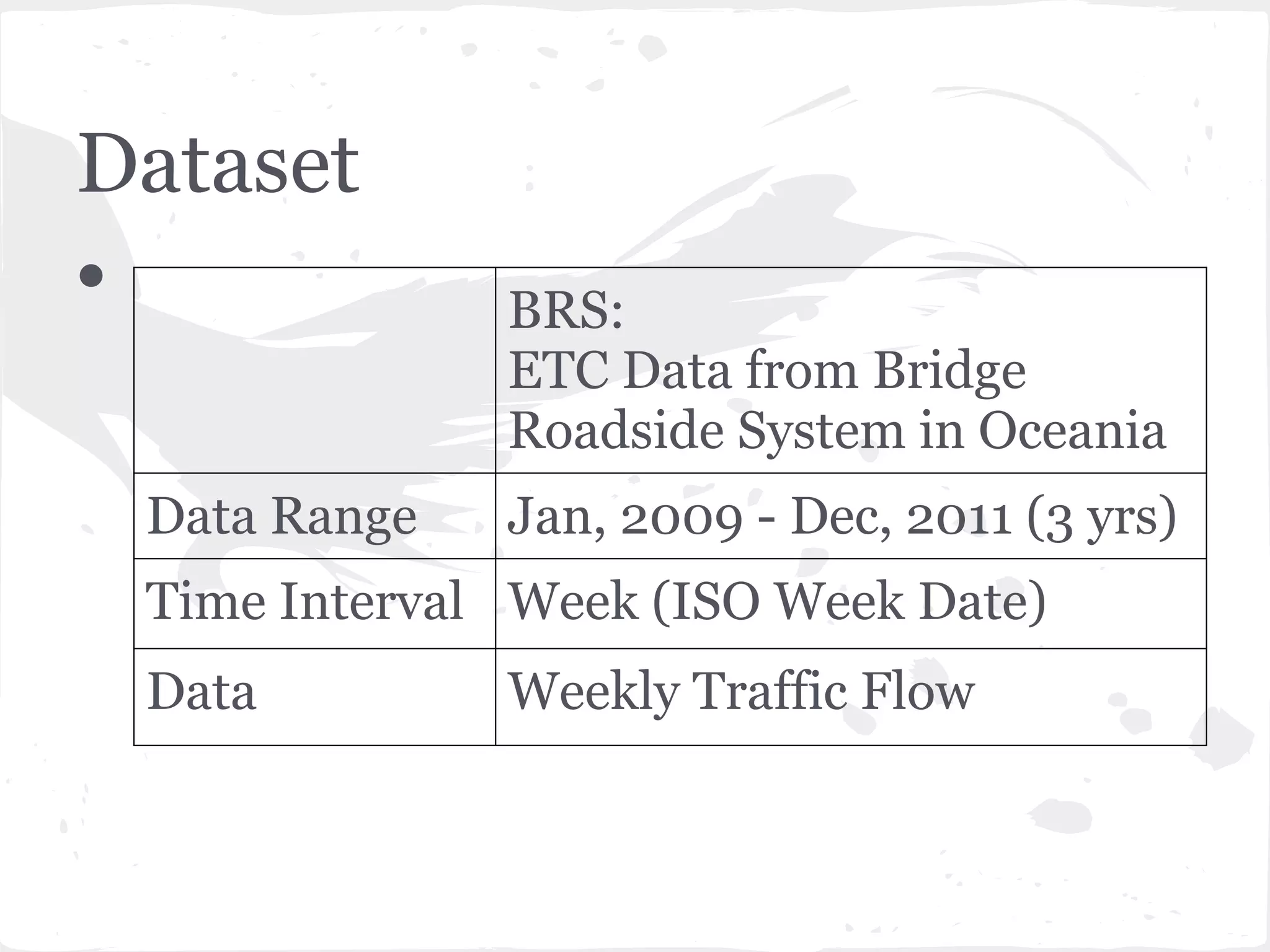
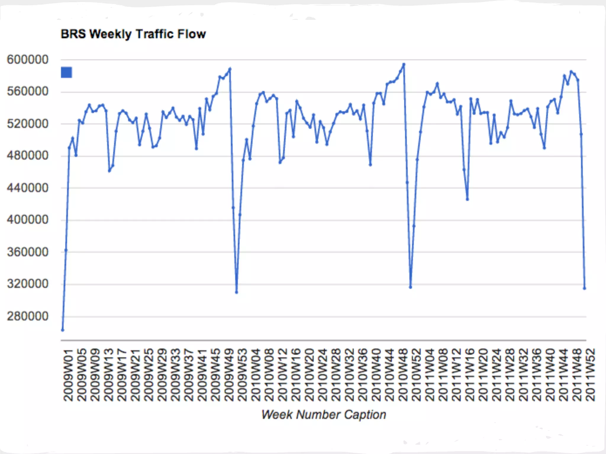
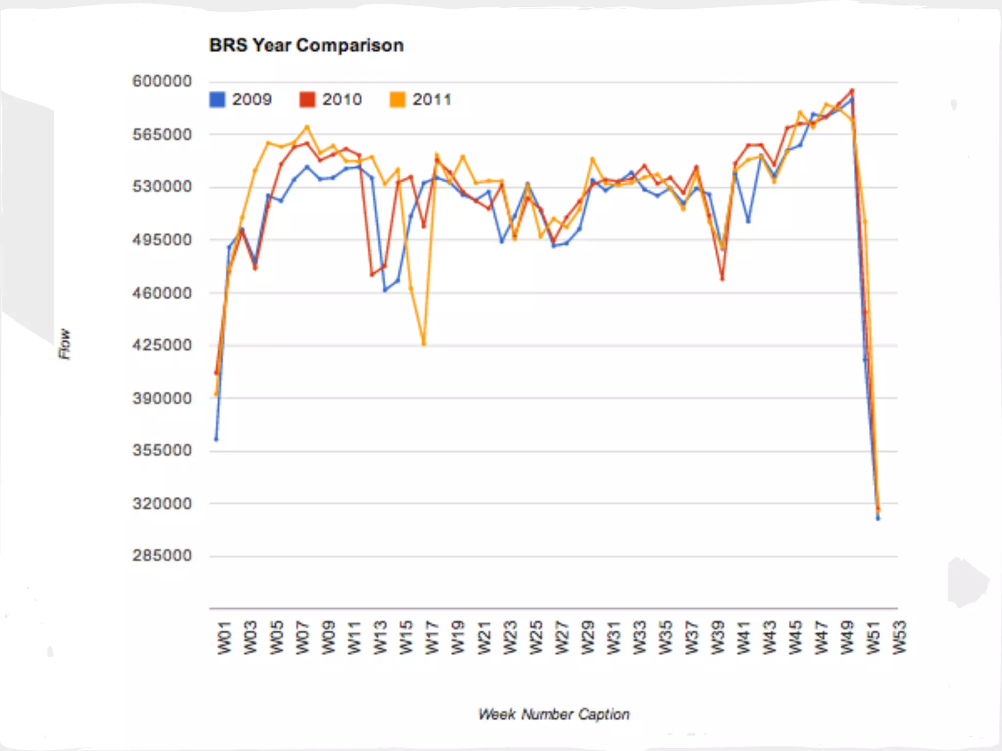
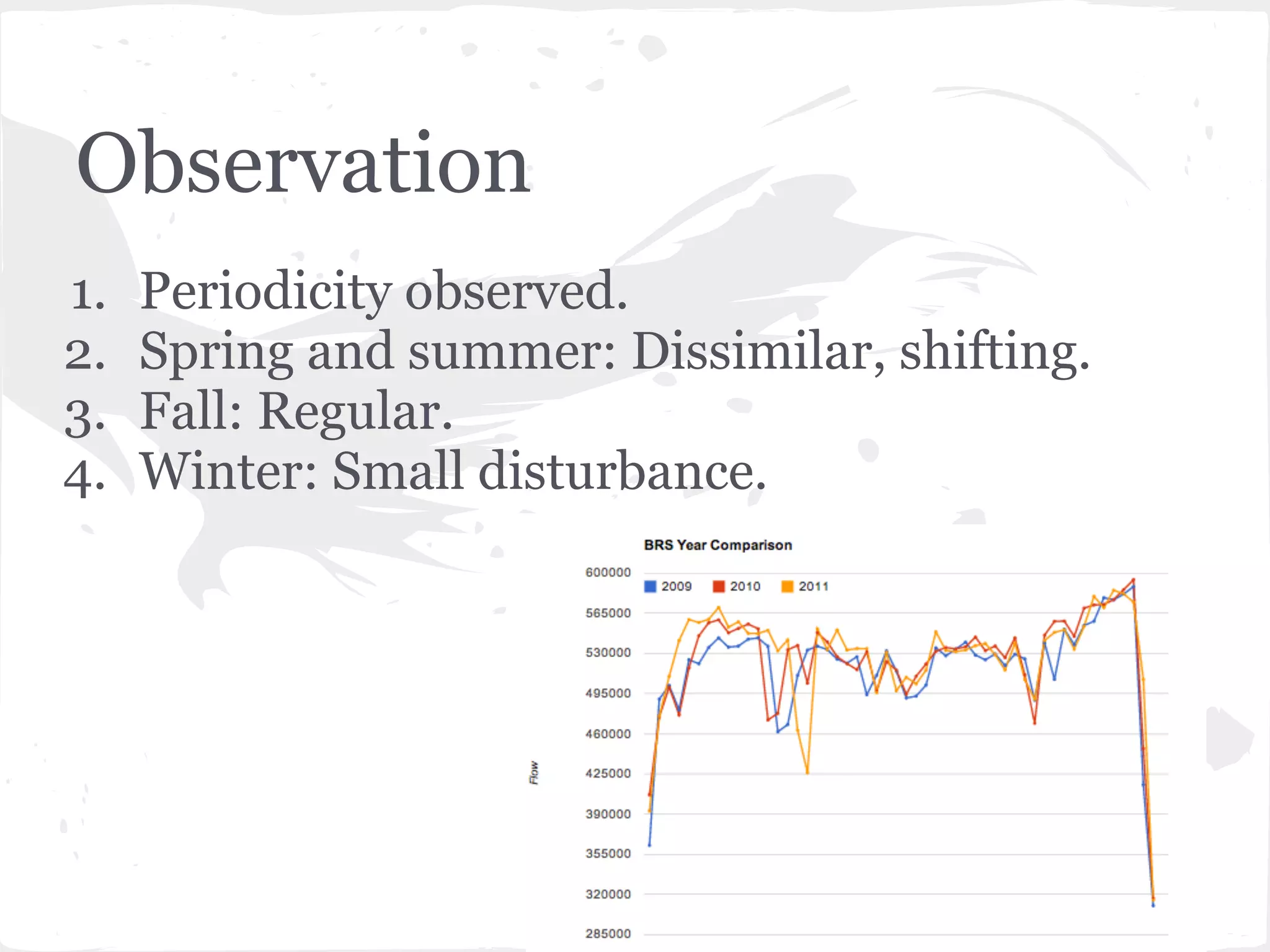
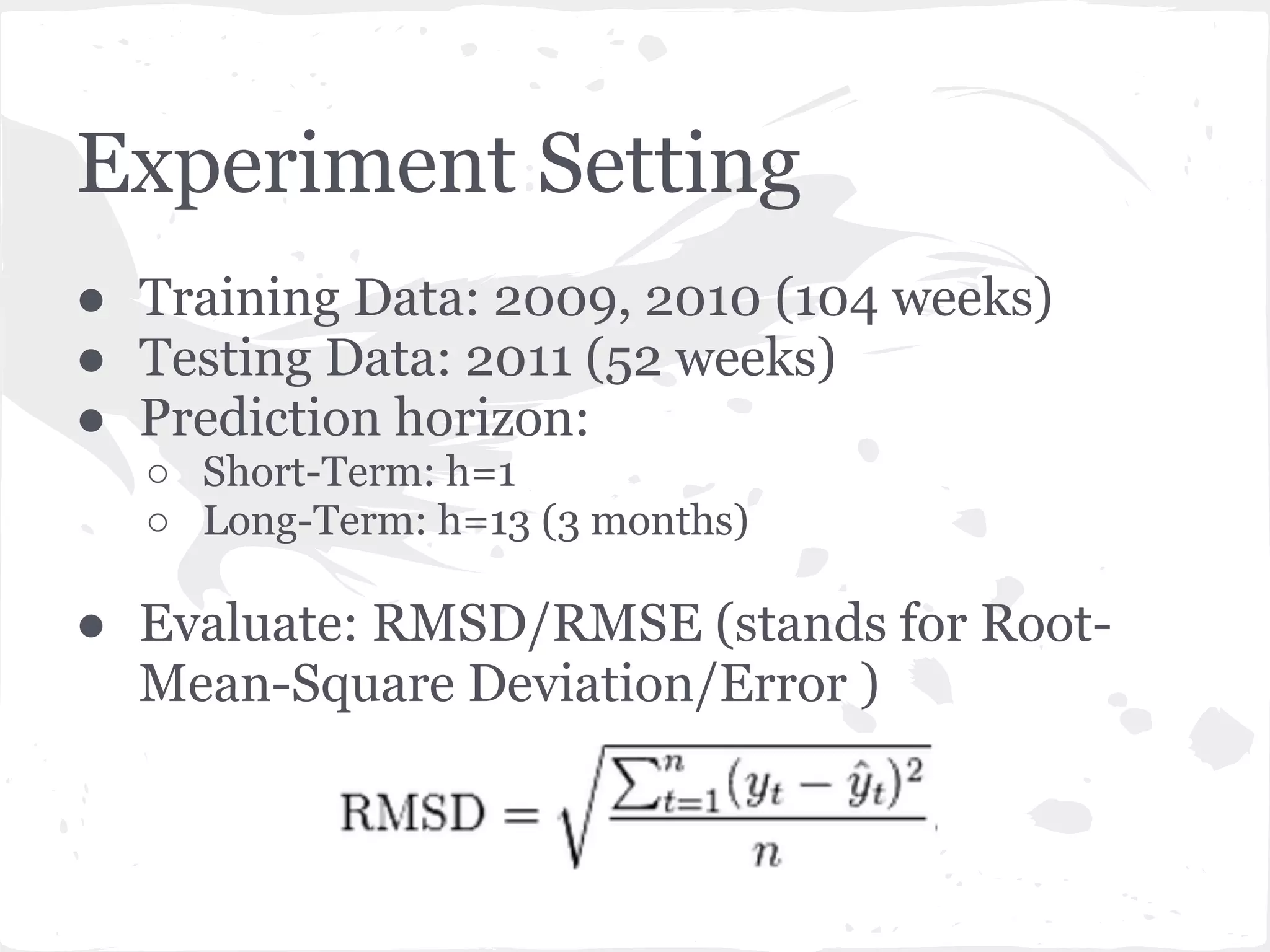
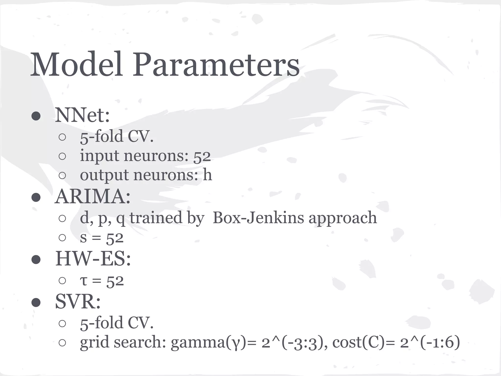

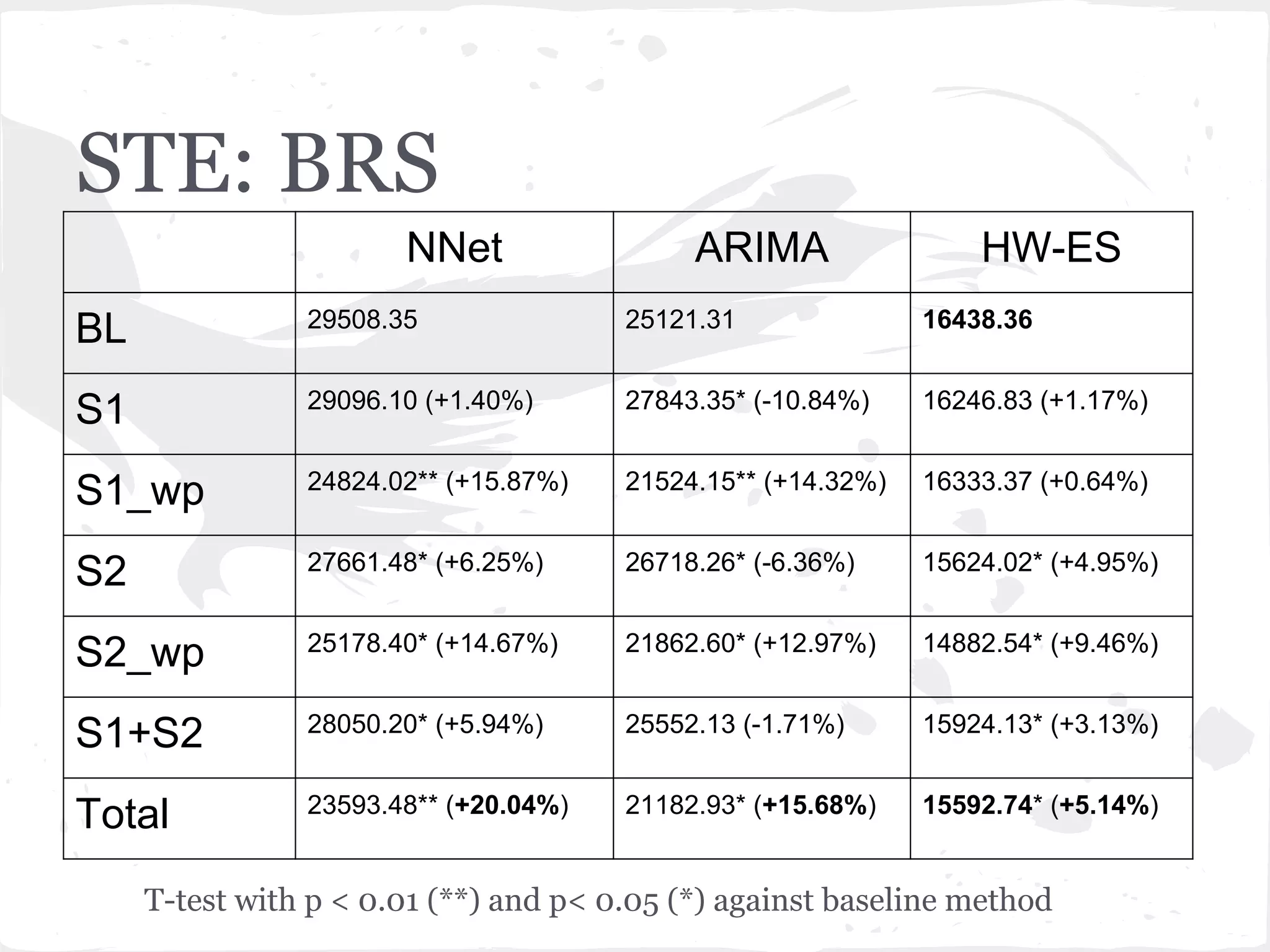
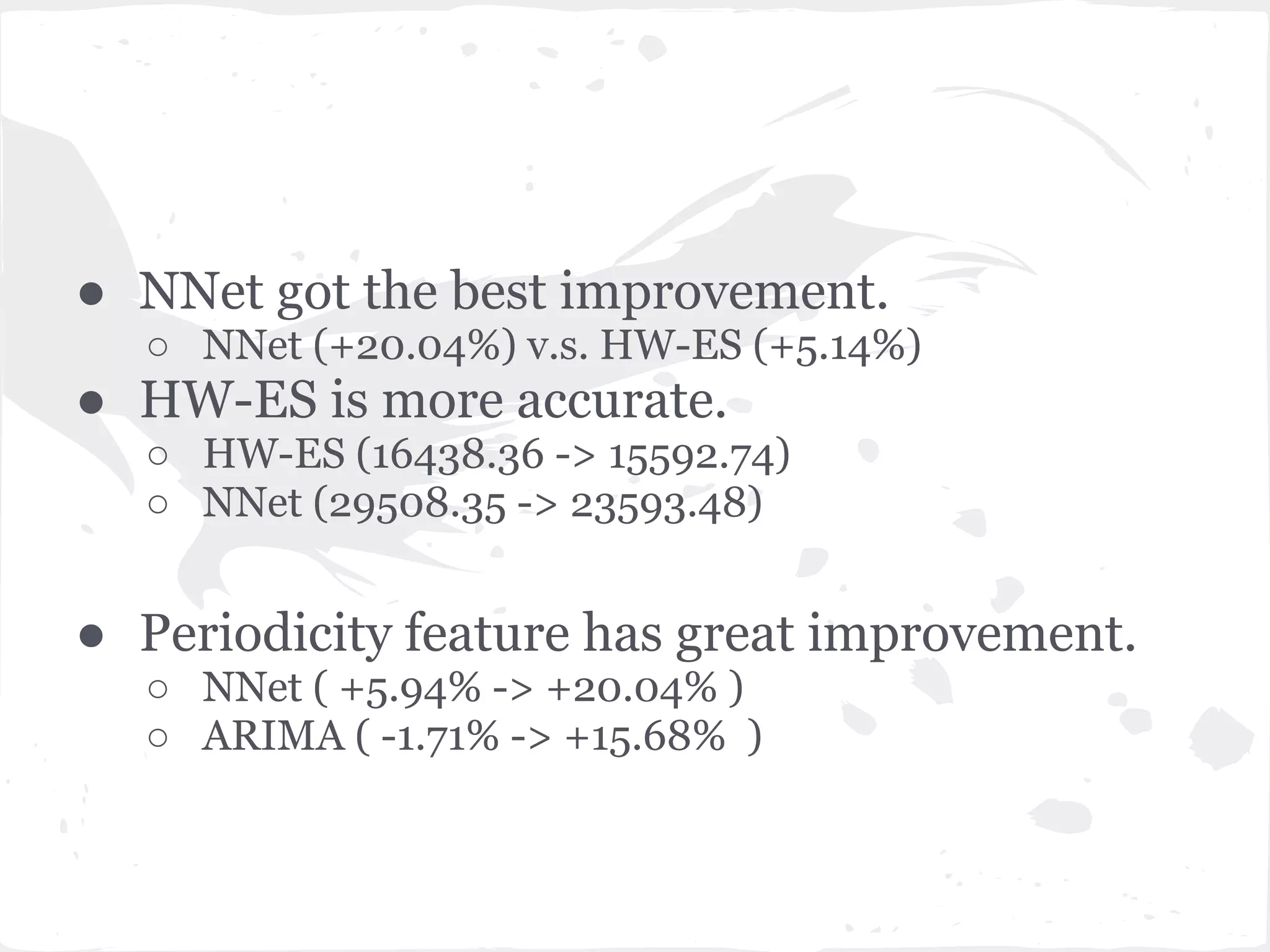
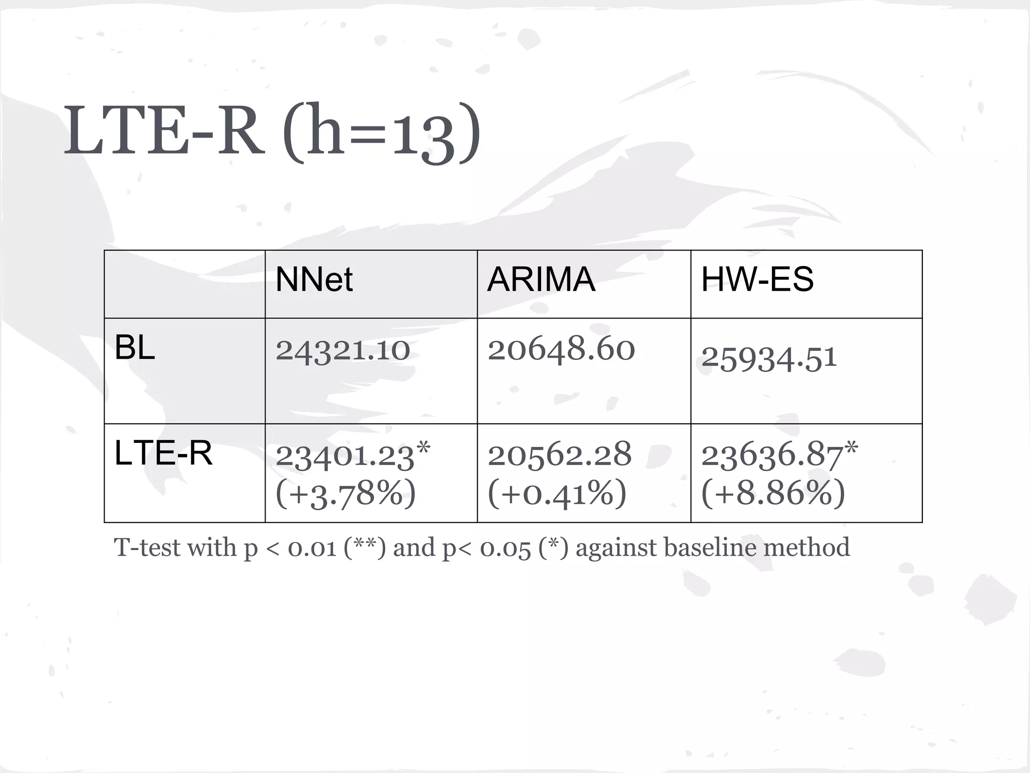
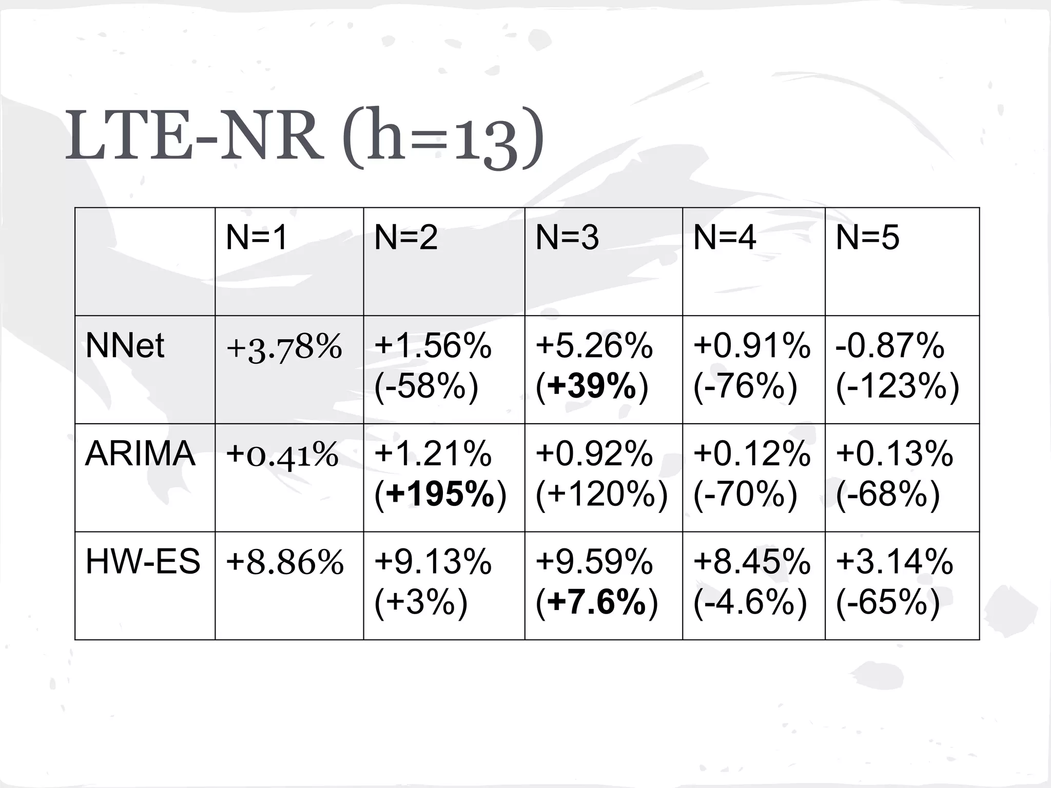

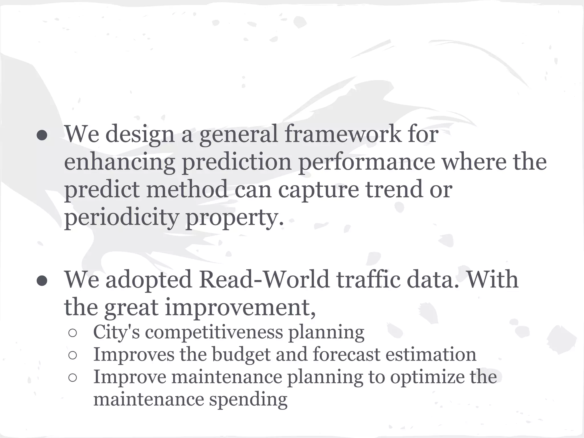

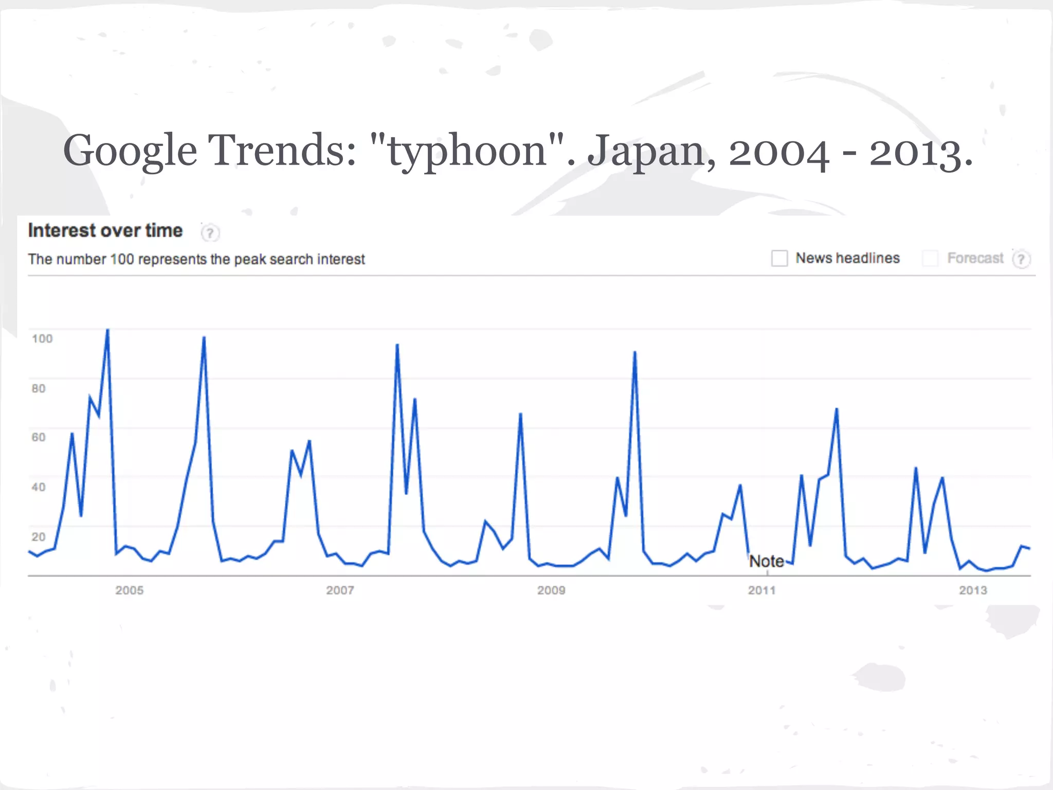
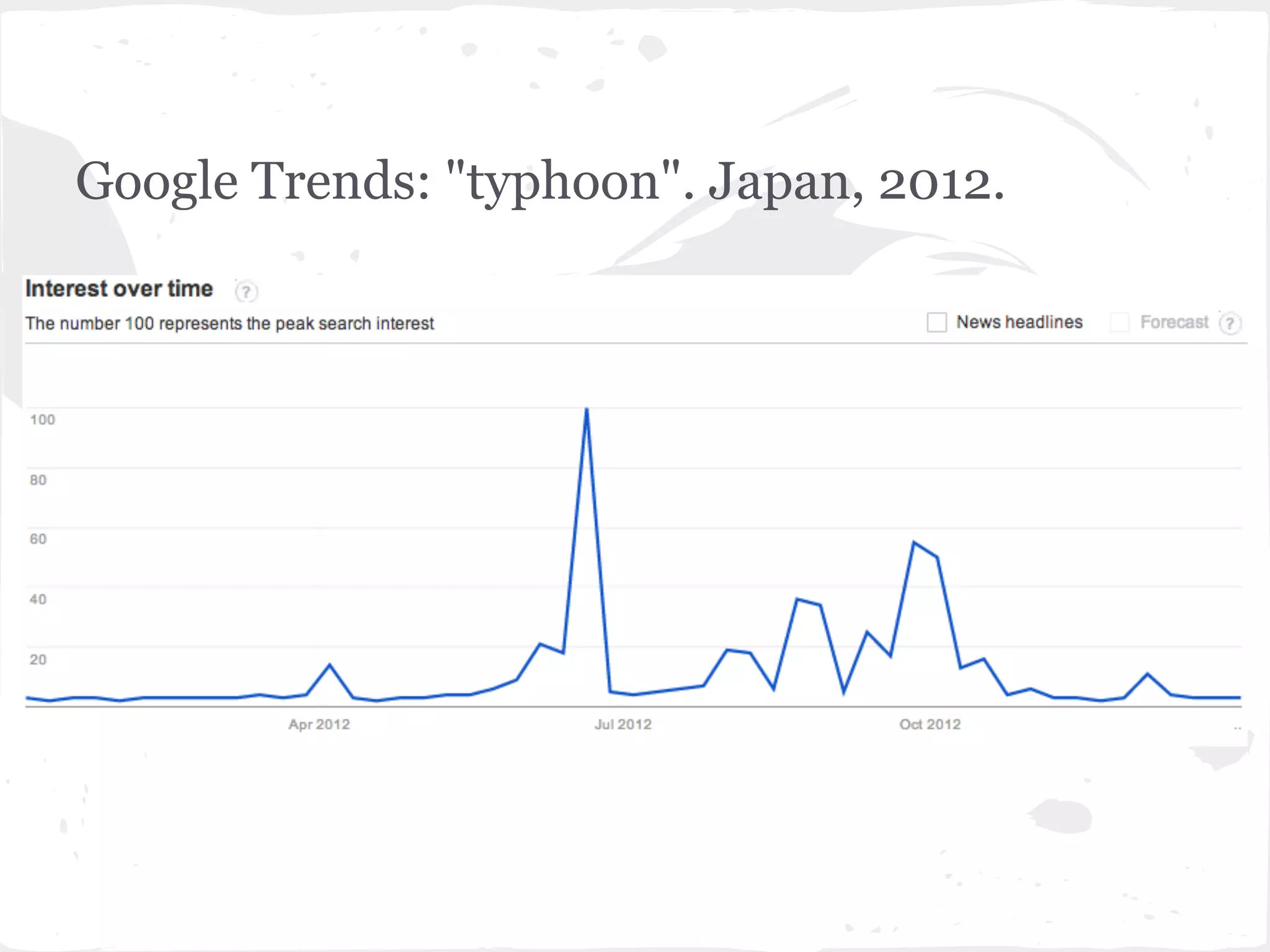
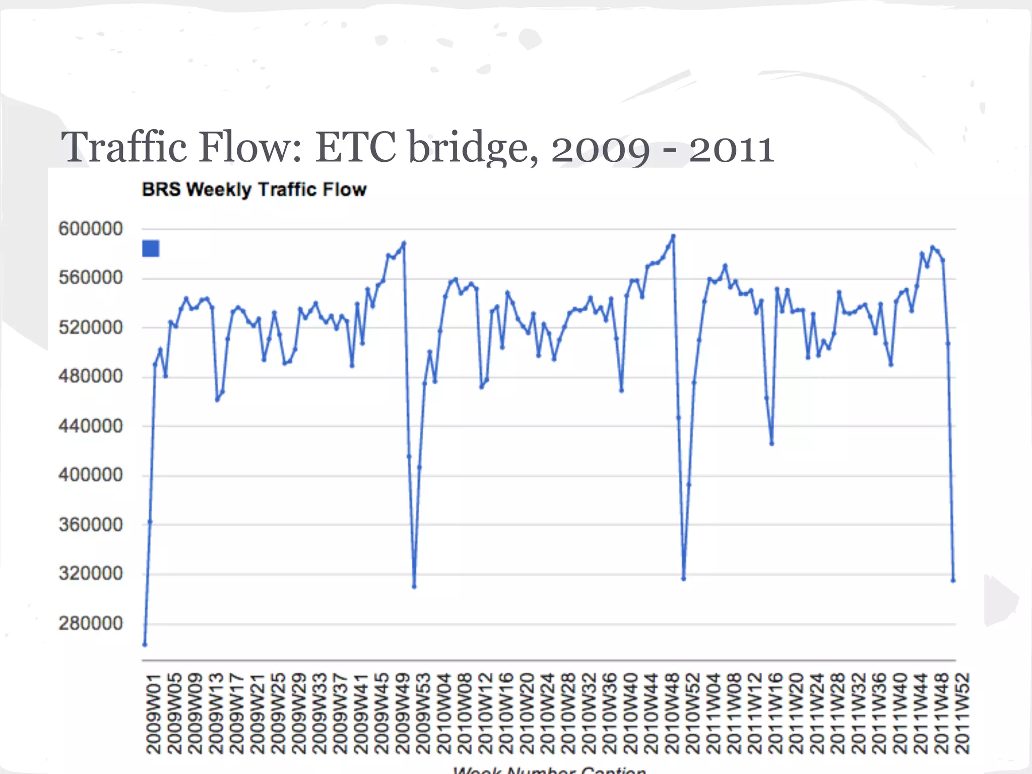
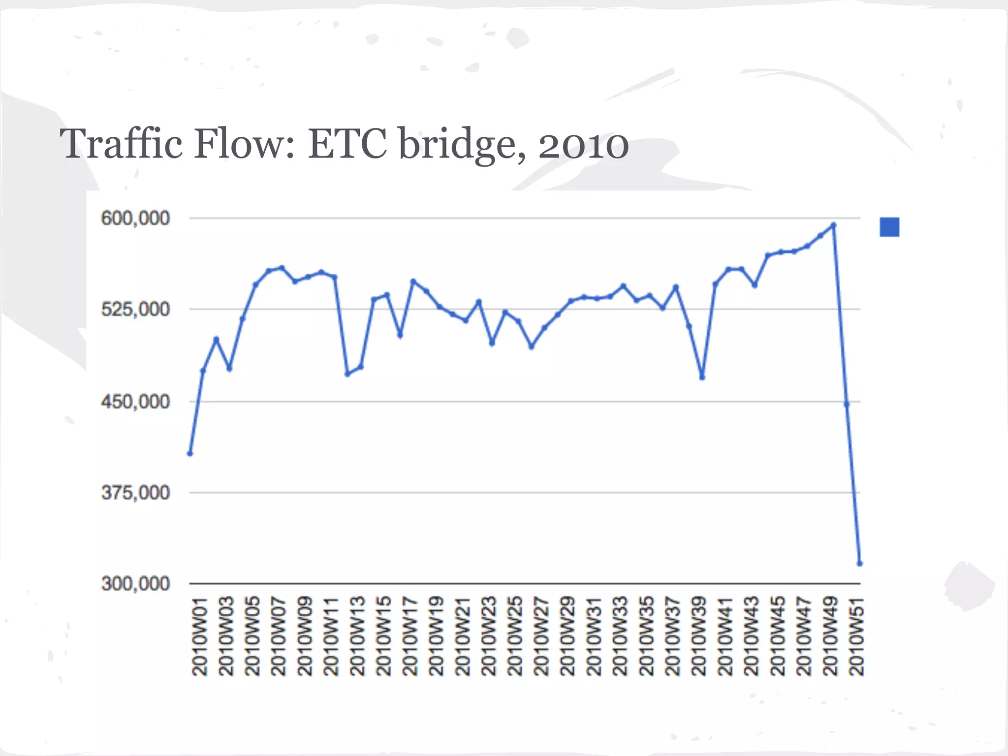
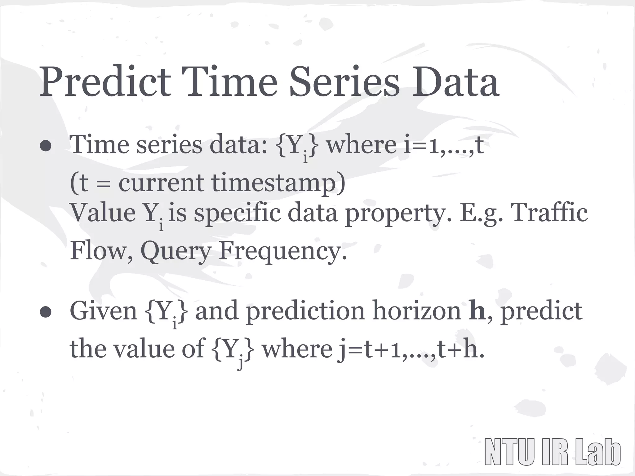
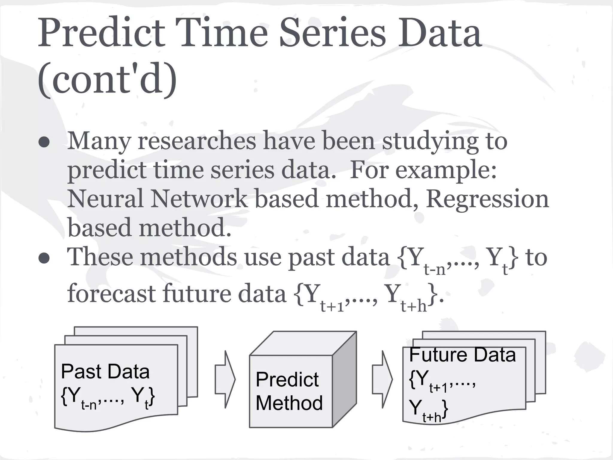
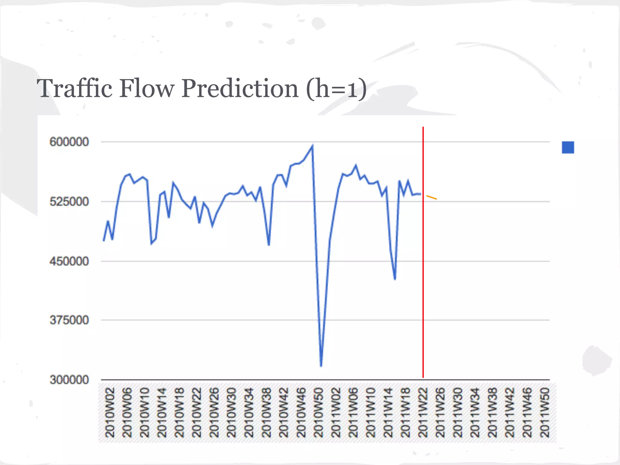
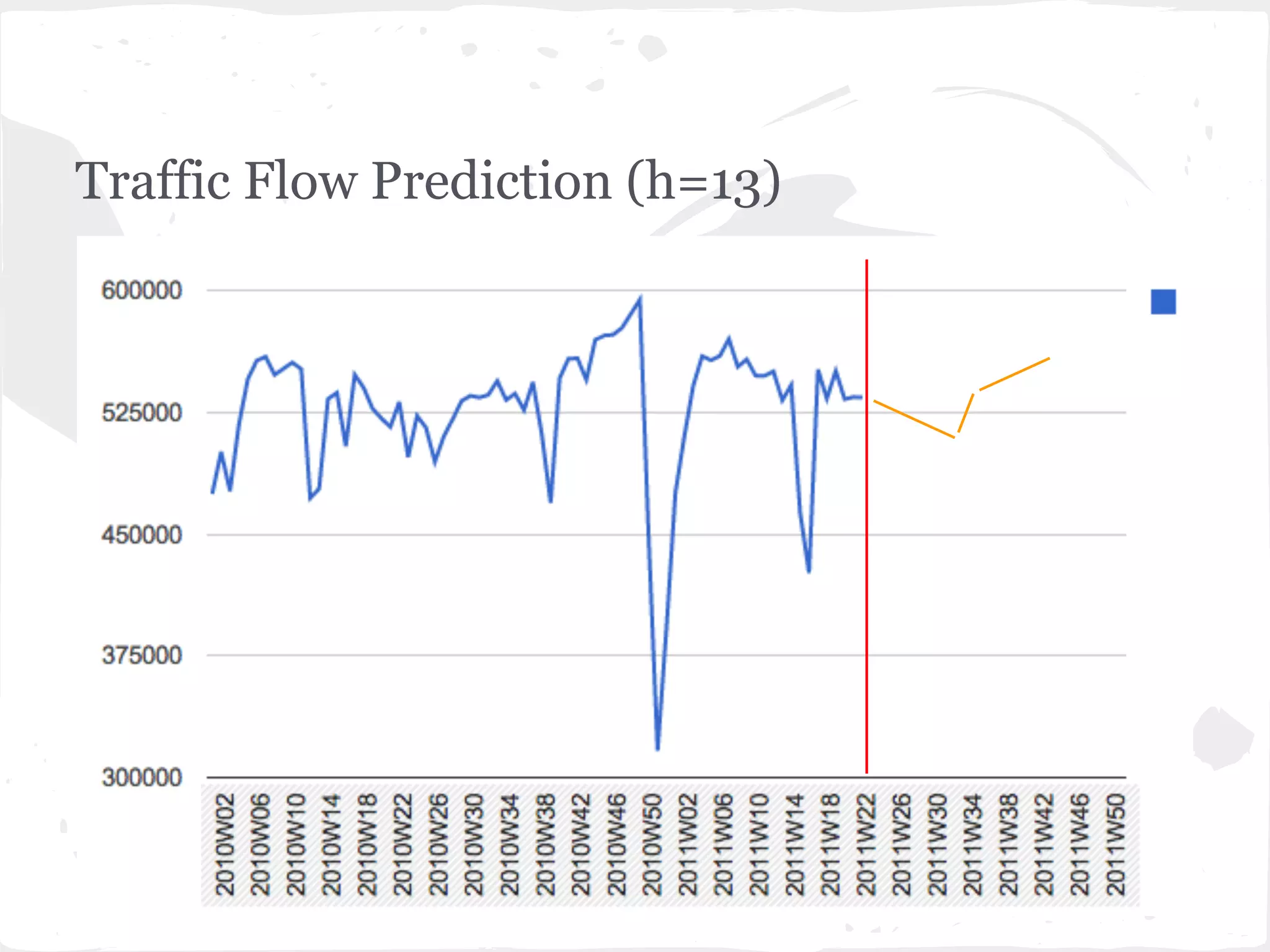
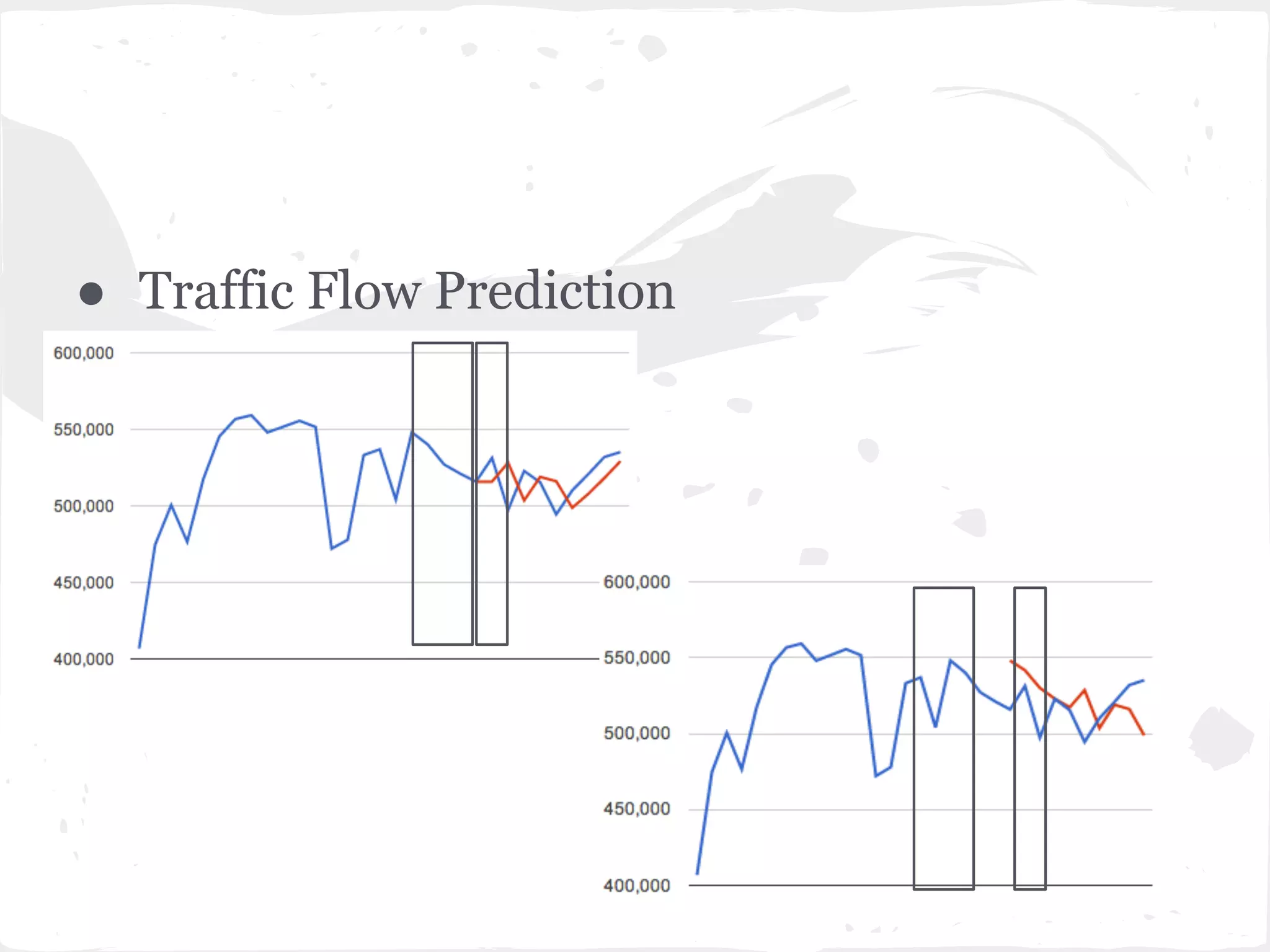
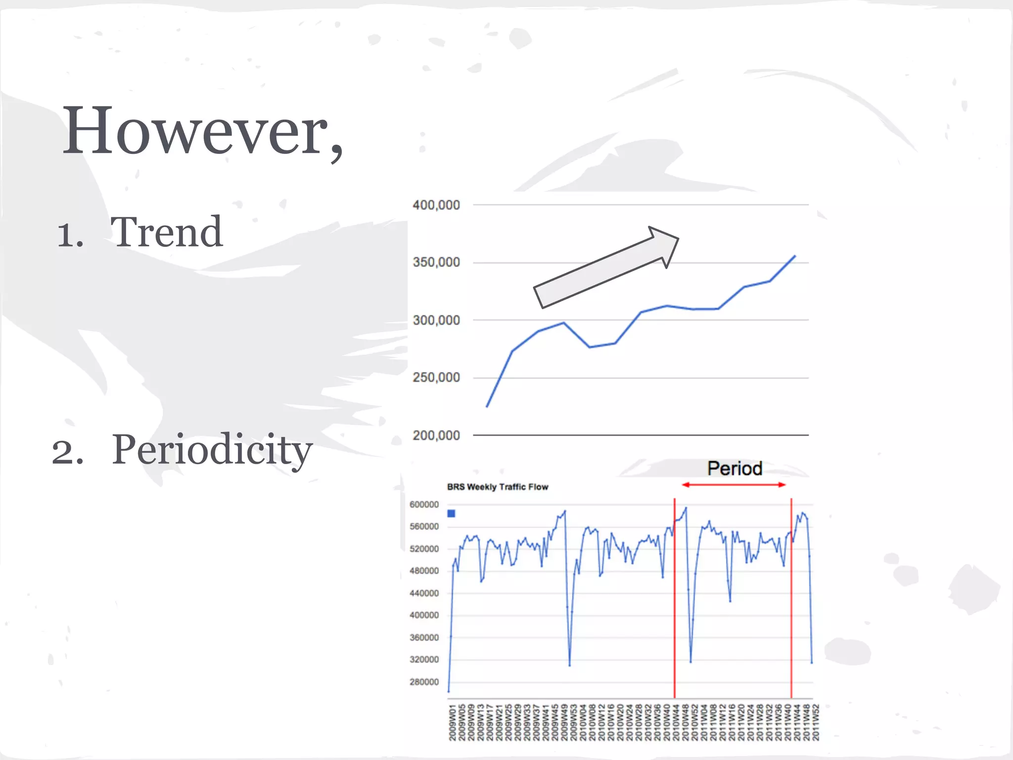
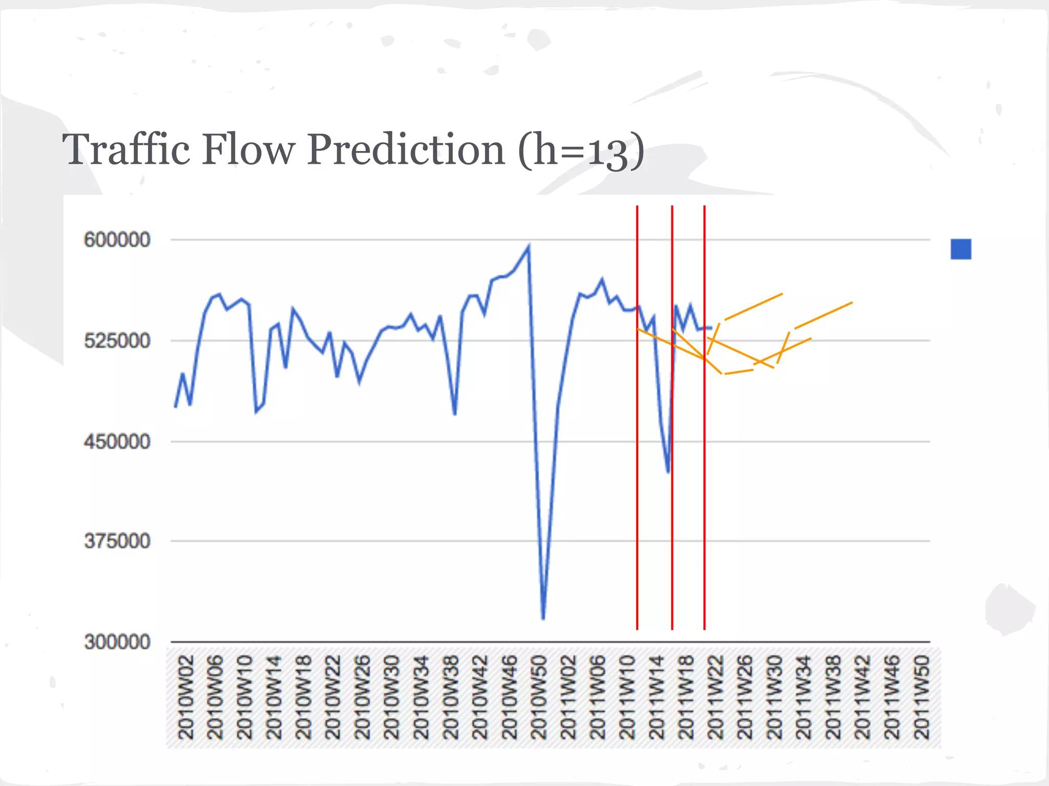
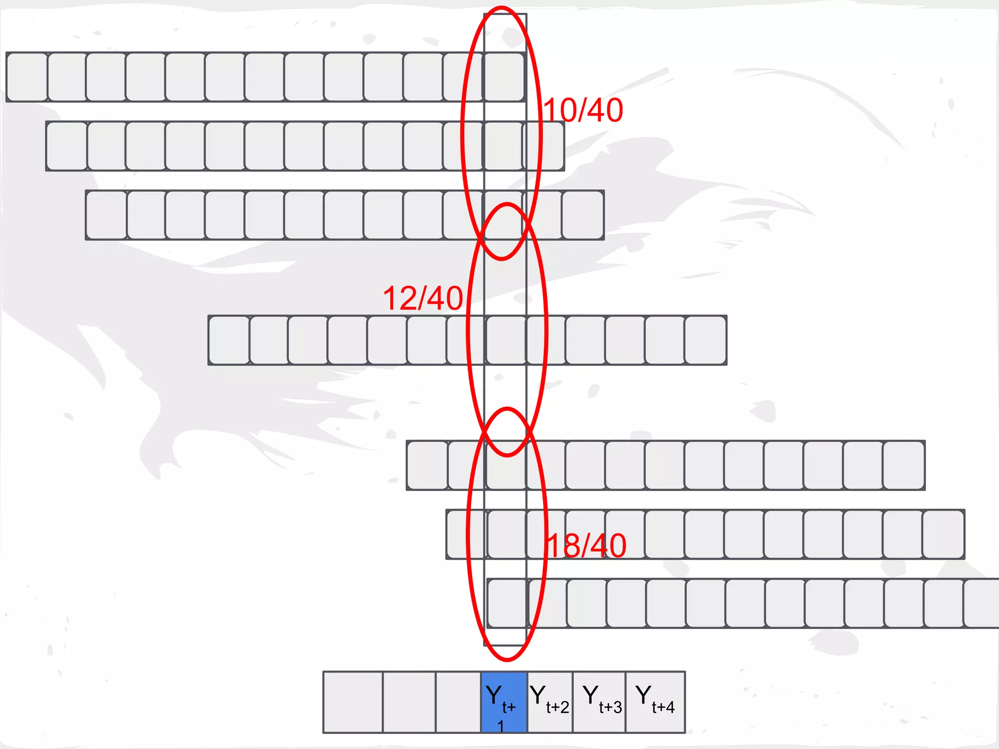
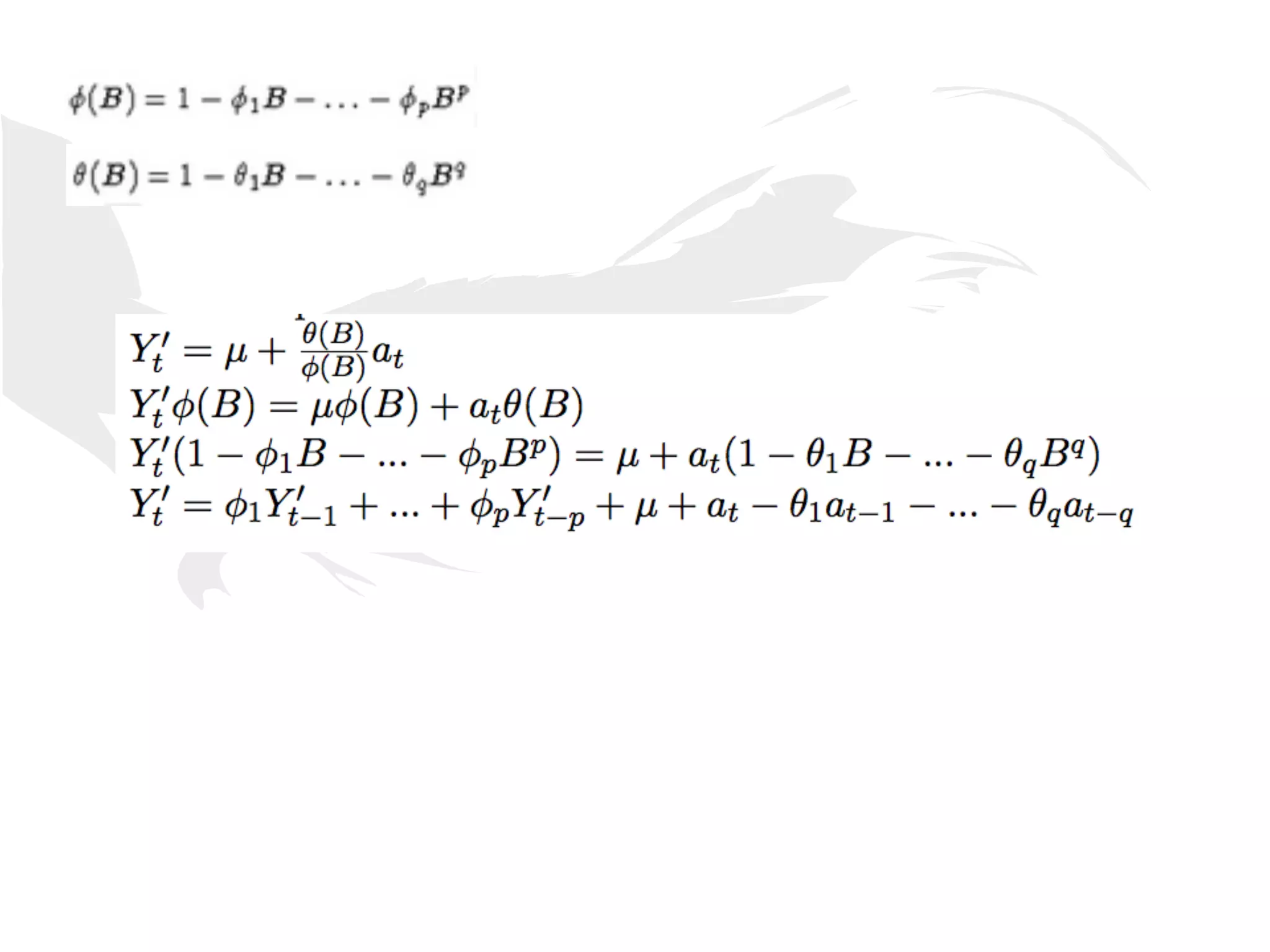
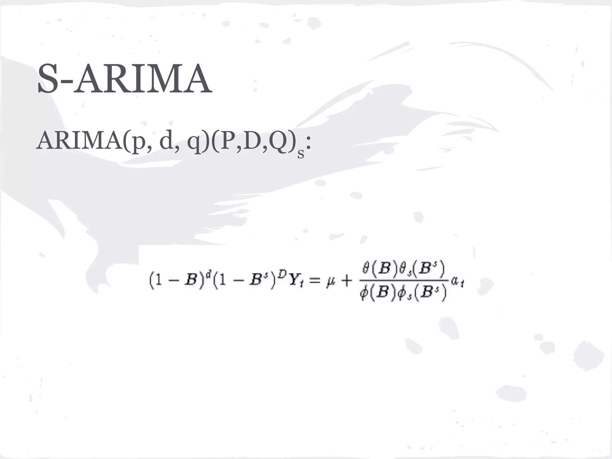
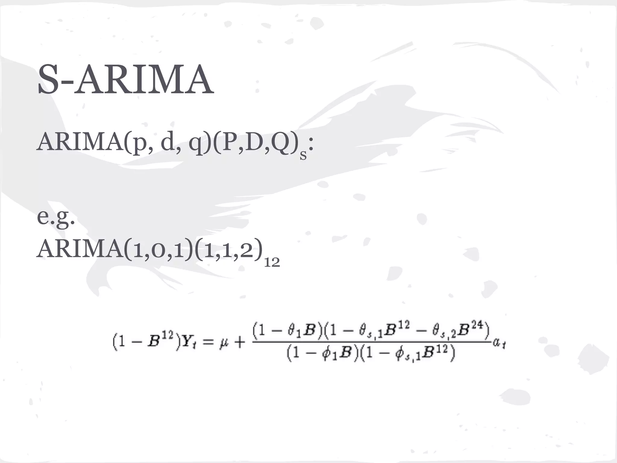
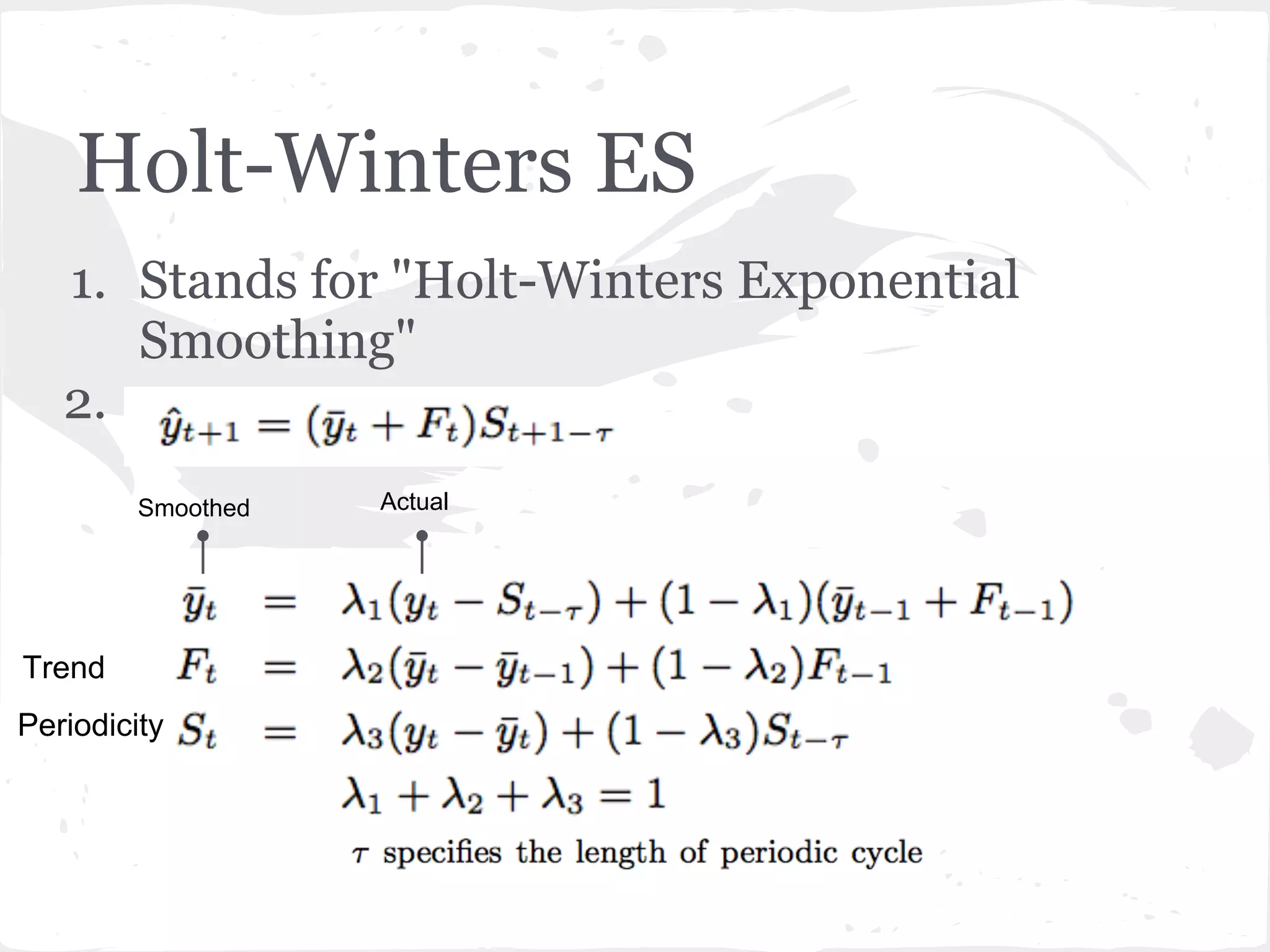
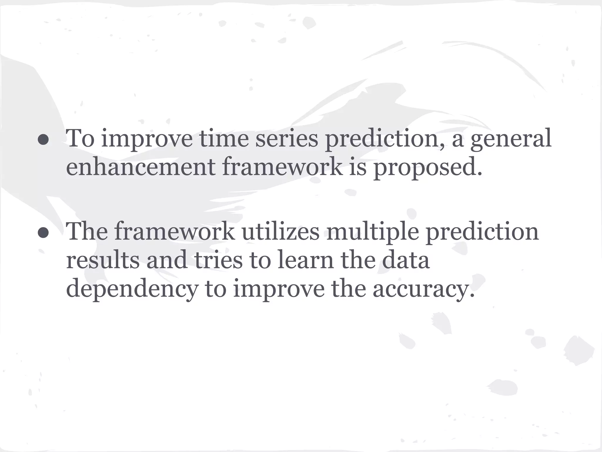
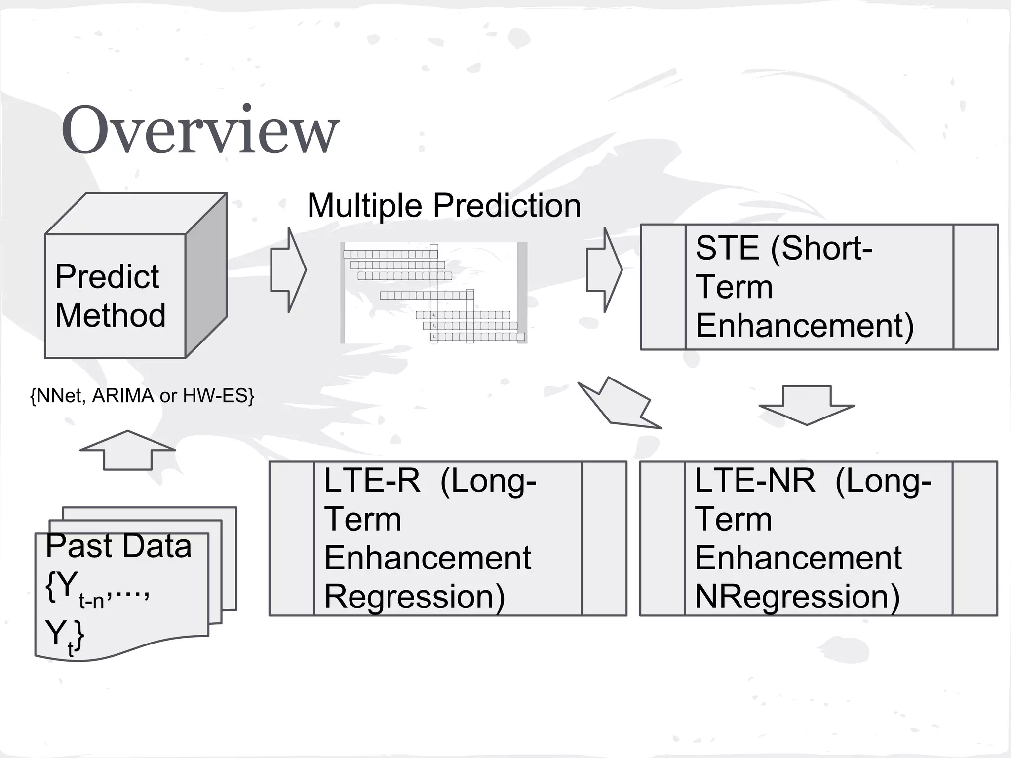
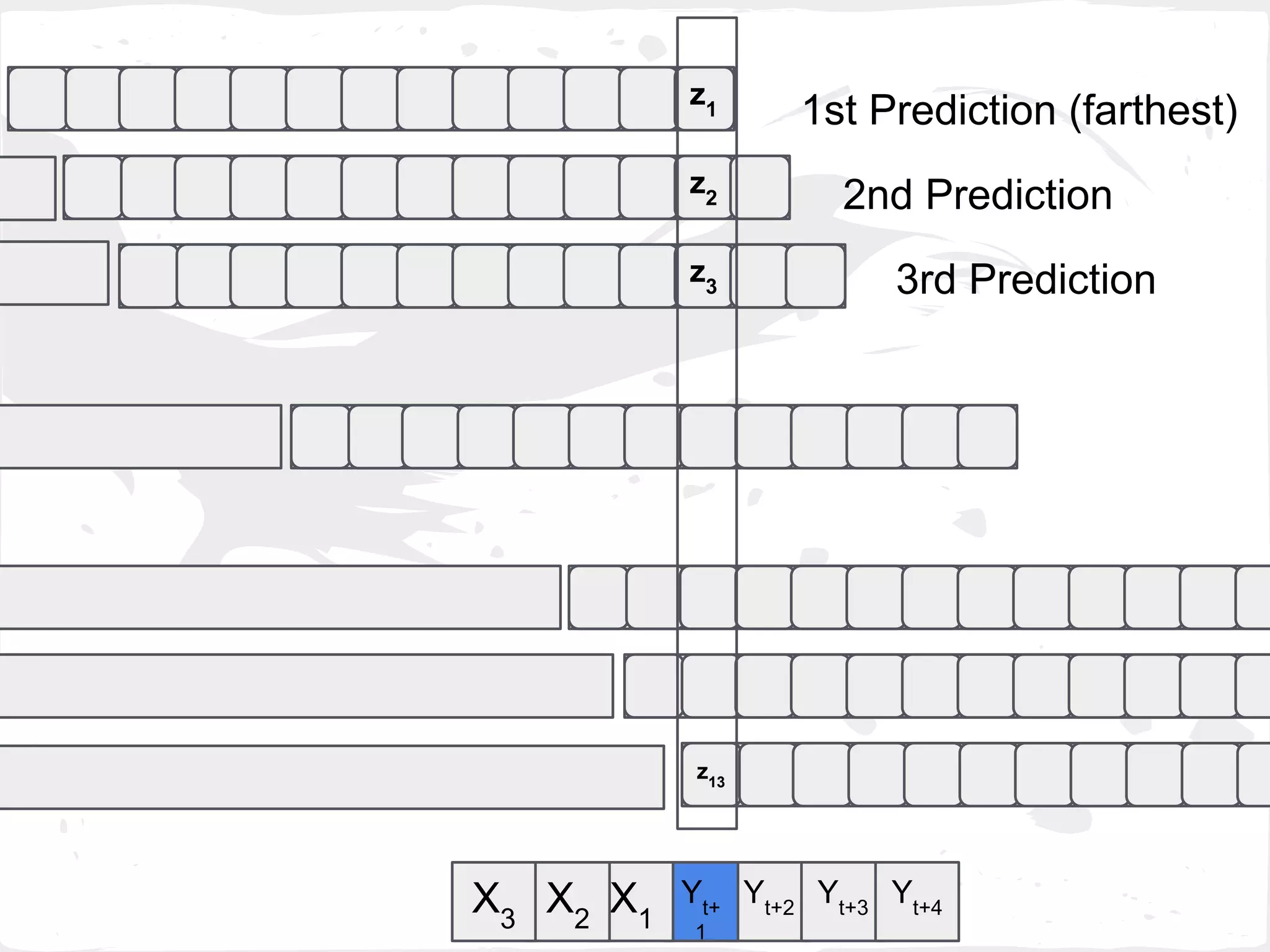
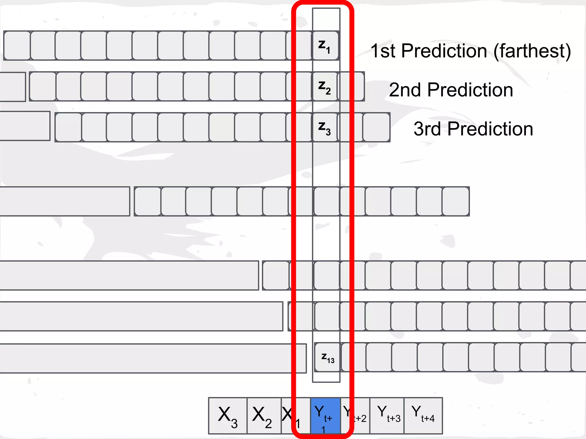
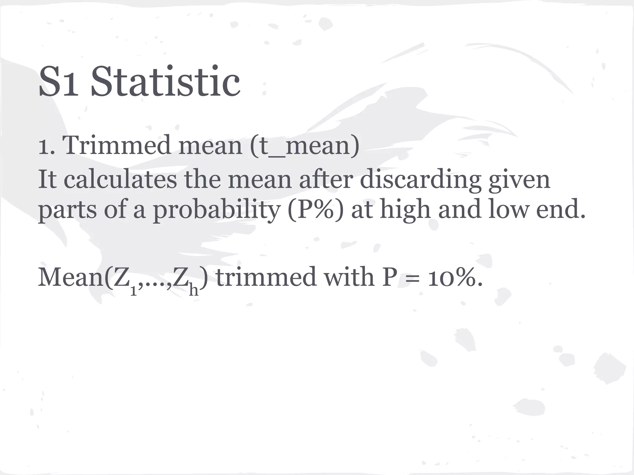
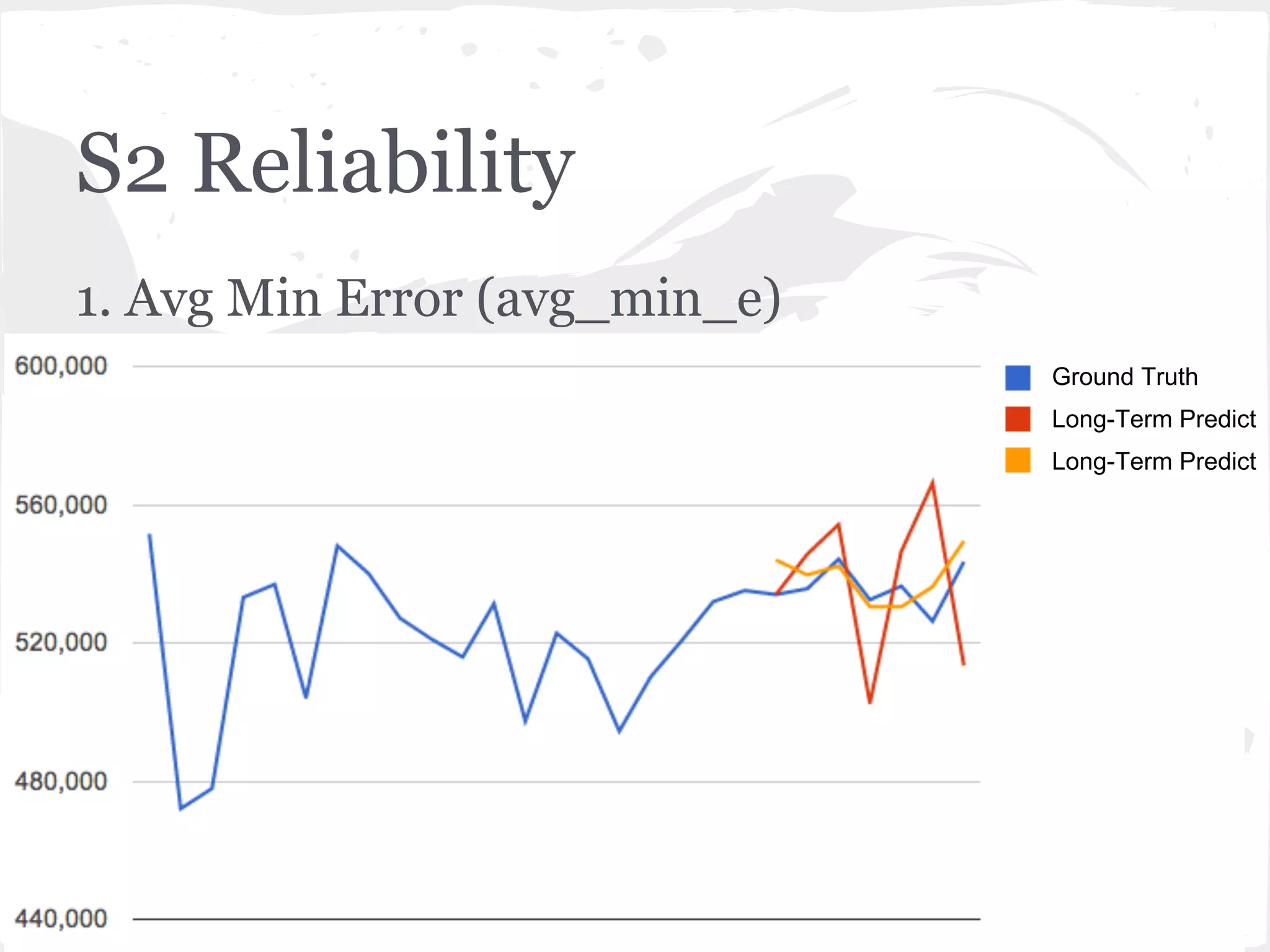
This document presents a general framework for enhancing time series prediction performance. It discusses using multiple predictions from a base method like neural networks, ARIMA or Holt-Winters to improve accuracy. Short-term enhancement uses support vector regression on statistic and reliability features of the multiple predictions to enhance 1-step ahead predictions. Long-term enhancement trains additional models on the short-term predictions to enhance longer-horizon predictions. The framework is evaluated on traffic flow data with prediction horizons of 1 week and 13 weeks.


![Digital Signal Processing[ECEG-3171]-Ch1_L04](https://cdn.slidesharecdn.com/ss_thumbnails/dspl4-180427094424-thumbnail.jpg?width=640&height=640&fit=bounds)


![[系列活動] Machine Learning 機器學習課程](https://cdn.slidesharecdn.com/ss_thumbnails/ml4ds02122017-170212005829-thumbnail.jpg?width=640&height=640&fit=bounds)


![[系列活動] 資料探勘速遊 - Session4 case-studies](https://cdn.slidesharecdn.com/ss_thumbnails/session4-case-studies-170114072124-thumbnail.jpg?width=640&height=640&fit=bounds)


![[DSC 2016] 系列活動:李祈均 / 人類行為大數據分析](https://cdn.slidesharecdn.com/ss_thumbnails/bspdatasci2016-jeremy-161029145502-thumbnail.jpg?width=640&height=640&fit=bounds)
![[系列活動] 給工程師的統計學及資料分析 123](https://cdn.slidesharecdn.com/ss_thumbnails/0114lckungtdsaprerequisite-170110090917-thumbnail.jpg?width=640&height=640&fit=bounds)

![[系列活動] Data exploration with modern R](https://cdn.slidesharecdn.com/ss_thumbnails/dataexplorationwithmodernr1221-161219044516-thumbnail.jpg?width=640&height=640&fit=bounds)