Download as PDF, PPTX

![Here, 𝑏 =
𝑋𝑌−
𝑋 𝑌
𝑛
𝑥2−
( 𝑥)2
𝑛
=
𝑋𝑌
𝑥2 =
17
28
= 4.18
𝑎 = 𝑌 − 𝑏𝑋 = 𝑌 =
𝑌
𝑛
=
609
7
= 87
[since 𝑥 = 0 ]
[since 𝑥 = 0 ]
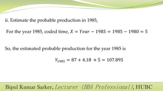
So the estimated equation of the linear trend is,
𝒀 𝒄 = 𝟖𝟕 + 𝟒. 𝟏𝟖 𝑿](https://image.slidesharecdn.com/timeserieschapter-07-171129181535/85/Time-series-Analysis-36-320.jpg)

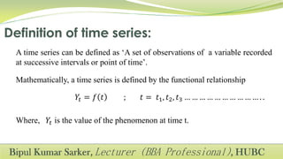
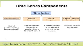
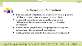
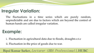
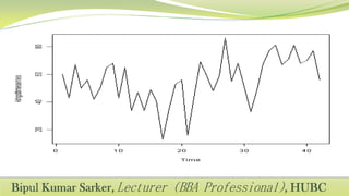
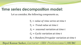
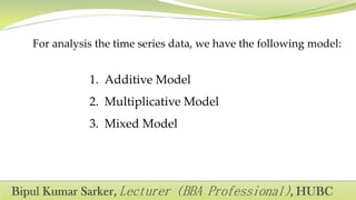
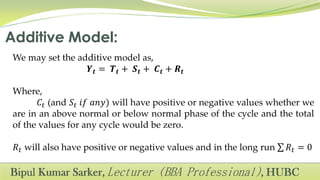
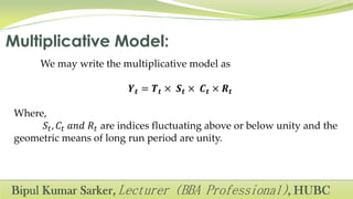
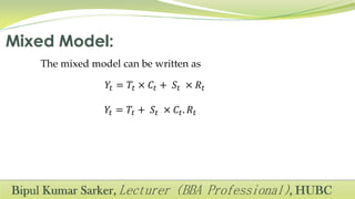
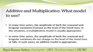
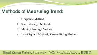
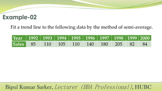
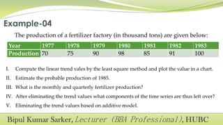
This document defines time series and its components. A time series is a set of observations recorded over successive time intervals. It has four main components: trend, seasonality, cycles, and irregular variations. Trend refers to the overall increasing or decreasing tendency over time. Seasonality refers to predictable changes that occur around the same time each year. Cycles have periods longer than a year. Irregular variations are random fluctuations. The document also discusses methods for analyzing time series components including additive, multiplicative, and mixed models.