The document discusses numerical integration using Gaussian quadrature. It describes one-point, two-point, and three-point Gaussian quadrature rules. For each rule, it provides the formula used to approximate a definite integral of a function over an interval by calculating a weighted sum of the function values at specified points. Examples are included to demonstrate applying the one-point, two-point, and three-point rules to evaluate definite integrals.

1. Numerical Integration
Gaussian integration one point, two point and three point method.

2. What is Integration?
 The process of measuring the area under a curve.
Where: f(x) is the integrand
a= lower limit of integration
b= upper limit of integration

b
a
dxxfI )(

3. Gaussian quadrature
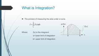
 In numerical analysis, a quadrature rule is an approximation of the definite
integral of a function, usually stated as a weighted sum of function values at
specified points within the domain of integration.
 An n-point Gaussian quadrature rule is a quadrature rule constructed to yield an
exact result for polynomials of degree 2n − 1 or less by a suitable choice of the
points xi and weights wi for i = 1, ..., n. The domain of integration for such a rule is
conventionally taken as [−1, 1], so the rule is stated as
 


n
i
ii xfwdxxf
0
1
1
)()(

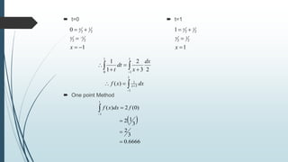
4. One-Point Gaussian Quadrature Rule
 Consider a function f(x) over interval [-1,1] with sampling point The point
one formula is
 The formula of one point Gaussian quadrature rule,


1
1
11 )()( xfwdxxf


1
1
)0(2)( fdxxf
11, wx

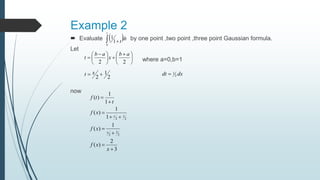
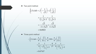
5. Two-Point Gaussian Quadrature Rule
 Consider a function f(x) over interval [-1,1] with sampling point and
The two point formula is,
 The formula of one point Gaussian quadrature rule,
)()()( 22
1
1
11 xfwxfwdxxf 














1
1 3
1
3
1
)( ffdxxf
21, xx
21,ww

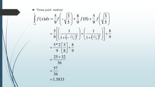
6. Three-Point Gaussian Quadrature Rule
 Consider a function f(x) over interval [-1,1] with sampling point and
The two point formula is,
 The formula of Three point Gaussian quadrature rule,
)()()()( 3322
1
1
11 xfwxfwxfwdxxf 

















5
3
9
5
)0(
9
8
5
3
-
9
5
)(
1
1
fffdxxf
321 ,, xxx
321 ,, www

7. Example 1
 Evaluate by one point , two point & Three point Gaussian
quadrature.
 Here,
 Using one point method
 Using Two point Method
dx
x

1
1
2
1
1
2
1
1
)(
x
xf


 
2
01
12
)0(2



 fdxxf
1
1
)(














1
1 3
1
3
1
)( ffdxxf
22
3
11
1
3
11
1














   3
1
3
1 1
1
1
1




5.14
6 

8.  Three point method

















5
3
9
5
)0(
9
8
5
3
-
9
5
)(
1
1
fffdxxf
   
5833.1
36
57
36
3225
9
8
8
5
9
2*5
9
8
1
1
1
1
9
5
2
5
3
2
5
3









































9. Example 2
 Evaluate by one point ,two point ,three point Gaussian formula.
Let
where a=0,b=1
now
 dt
t 
1
0
1
1





 





 

22
ab
x
ab
t
2
1
2
 xt dxdt 2
1
3
2
)(
1
)(
1
1
)(
1
1
)(
2
3
2
2
1
2








x
xf
xf
xf
t
tf
x
x

10.  t=0
 One point Method
 t=1
1
0
2
1
2
2
1
2




x
x
x
1
1
2
1
2
2
1
2



x
x
x
 




1
0
1
1
23
2
1
1 dx
x
dt
t


1
1
3
1
)( dxxf x


1
1
)0(2)( fdxxf
 
6666.0
3
2
3
12




11.  Two point method
 Three point method














1
1 3
1
3
1
)( ffdxxf
   
6923.0
331
3
331
3
3
1
3
1
3
1
3
1


























 
5
3
9
5
)0(
9
8
5
3
-
9
5
)(
1
1
fffdxxf
67167.0
3
5
3
1
9
5
27
8
3
5
3
1
9
5














