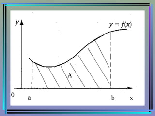
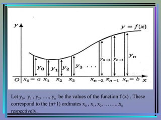
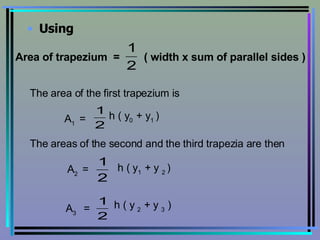
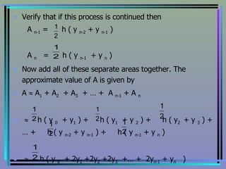
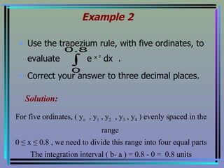
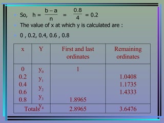
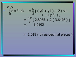
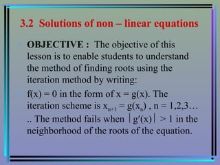
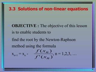
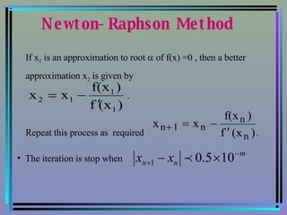
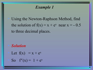
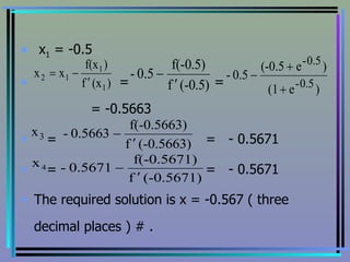
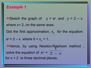
The document discusses numerical methods for approximating integrals and solving non-linear equations. It introduces the trapezium rule for approximating integrals and provides examples of using the rule. It then discusses iterative methods like the iteration method and Newton-Raphson method for finding approximate roots of non-linear equations, providing examples of applying each method. The objectives are to enable students to use the trapezium rule and understand solving non-linear equations using iterative methods.

1. CHAPTER 3 NUMERICAL METHOD

2. 3.1 The Trapezium Rule OBJECTIVES : The objectives of this lesson are to enable students to a) derive the trapezium rule by dividing the area represented by dx into n ( n  7 ) trapezium each with width h. b) use the trapezium rule to approximate

3. Introduction What happens when a mathematical function cannot be integrated ? In these cases a numerical method can be used to find an approximate value for the integral As the definite integral is a number which represents the area between y = f (x) , the x-axis and the lines x = a and x =b .

4. Therefore , even if cannot be found, approximate value for can be found by evaluating the appropriate area using another method. The two common methods are the trapezium rule and Simpson’s rule. However, here we will discuss the trapezium rule as requested by our syllabus .

5. The trapezium rule This method divides the area A under the curve y = f(x) is into n vertical strips. The width of each strip is h. The area under the curve  sum of areas of n trapezia. Note :  approximately equal to

7. Let y 0 , y 1 , y 2 , …., y n be the values of the function f (x) . These correspond to the (n+1) ordinates x 0 , x 1 , x 2 , ……..,x n respectively.

8. Using Area of trapezium = ( width x sum of parallel sides ) The area of the first trapezium is A 1 = h ( y 0 + y 1 ) The areas of the second and the third trapezia are then A 2 = h ( y 1 + y 2 ) A 3 = h ( y 2 + y 3 )

9. Verify that if this process is continued then A n-1 = h ( y n-2 + y n-1 ) A n = h ( y n-1 + y n ) Now add all of these separate areas together. The approximate value of A is given by A  A 1 + A 2 + A 3 + … + A n-1 + A n  h ( y 0 + y 1 ) + h ( y 1 + y 2 ) + h ( y 2 + y 3 ) + … + h ( y n-2 + y n-1 ) + h ( y n-1 + y n )  h ( y 0 + 2y 1 +2y 2 +2y 3 +… + 2y n-1 + y n )

10. This method of approximating the area under a curve by n trapezia of equal width h is called the trapezium rule, and the result can be summarized as : dx  h  y 0 + y n + 2 ( y 1 + y 2 + … + y n-1 )  where h = and y r = f ( x r )

11. Example 1 Evaluate dx using 5 strips by the trapezium rule. Notation: Working must have 4 or more decimal places. Solution The integration interval ( b- a ) = 6 –1 = 5 units So h = = = 1

12. The value of x at which y is calculated are : 1, 2, 3, 4, 5, 6 Tabulating the results as follows help the final calculation : 4.787 1.792 Totals 0.693 1.099 1.386 1.609 0 1.792 y 0 y 1 y 2 y 3 y 4 y 5 1 2 3 4 5 6 Remaining ordinates First and last ordinates y X

13. dx   ( y 0 + y 5 ) + 2 ( y 1 +… +y 4 )  =  1.792 + 2 ( 4.787 )  = 5.683

14. Example 2 Use the trapezium rule, with five ordinates, to evaluate e x ² dx . Correct your answer to three decimal places. Solution: For five ordinates, ( y o , y 1 , y 2 , y 3 , y 4 ) evenly spaced in the range 0 ≤ x ≤ 0.8 , we need to divide this range into four equal parts The integration interval ( b- a ) = 0.8 - 0 = 0.8 units

15. So, h = = = 0.2 The value of x at which y is calculated are : 0 , 0.2, 0.4, 0.6 , 0.8 3.6476 2.8965 Totals 1.0408 1.1735 1.4333 1 1.8965 y 0 y 1 y 2 y 3 y 4 0 0.2 0.4 0.6 0.8 Remaining ordinates First and last ordinates Y x

16. e x ² dx ≈  ( y0 + y4 ) + 2 ( y1 +… +y 3 )  =  2.8965 + 2 ( 3.6476 )  = 1.0192 = 1.019 ( three decimal places )

17. 3.2 Solutions of non – linear equations OBJECTIVE : The objective of this lesson is to enable students to understand the method of finding roots using the iteration method by writing: f(x) = 0 in the form of x = g(x). The iteration scheme is x n+1 = g(x n ) , n = 1,2,3….. The method fails when  g  (x)  > 1 in the neighborhood of the roots of the equation.

18. Introduction Many equations cannot be solved exactly, but various methods of finding approximate numerical solutions exist. The most commonly used methods have two main parts: (a) finding an initial approximate value (b) improving this value by an iterative process

19. Initial Values: The initial value of the roots of f(x) = 0 can be located approximately by either a graphical or an algebraic method. Graphical Method: Either (a) Plot ( or sketch ) the graph of y = f(x). The real roots are the points where the curve cuts the x axis. Or (b) Rewrite f(x) = 0 in the form F(x) = G(x). Plot ( or sketch ) y =F(x) and y = G(x). The real roots are at the points where these graphs intersect.

20. Example 1 Find the approximate value of the equation ln x + x - 4 = 0 by using the graphical method. y = 4-x y 0 1 2 3 4 the intersection is at x  2.9 x y y = ln x

21. Algebraic Method Find two values a and b such that f(a) and f(b) have different signs. At least one root must lie between a and b if f(x) is continuous. If more than one root is suspected between a and b, sketch a graph of y = f(x).

22. Iterative Method All iterative methods follow the same basic pattern. A sequence of approximations x 1 , x 2 , x 3 , x 4 ….. is found , each one closer to the root  of f(x)=0. Each approximation is found from the one before it using a specified method. The process is continued until the required accuracy is reached. Two methods we have to discuss are Iteration Method and Newton-Raphson Method.

23. Iteration Method Rewrite the equation f(x) = 0 in the form x = g(x). If the initial approximation is x 1 , then calculate x 2 = g(x 1 ) x 3 = g(x 2 ) x 4 = g(x 3 ) and so on ….. This method fails if  g  (x)  > 1 near the root. So, the value of  g  (x1)  should be < 1.

24. Example 2 Using the iteration method, find the solution of f(x) = x + e x near x = -0.6 to three decimal places. Solution Iteration method Write the given equation as x = - e x  x = g(x) g (x) = - e x g  (x) = - e x ,  g  (-0.6)  =  -e-0.6  = 0.5488 ( < 1 )

25. x 1 = -0.6 x 2 = -e-0.6 = -0.5488 x 3 = -e-0.5488 = -0.5453 x 4 = -e-0.5453 = -0.5797 x 5 = -e-0.5797 = -0.5601 x 6 = -e-0.5601 = -0.5712 x 7 = -e-0.5712 = -0.5648 x 8 = -e-0.5648 = -0.5684 x 9 = -e-0.5684 = -0.5664 x 10 = -e-0.5664= -0.5676 x 11 = -e-0.5676 = -0.5668 x 12 = -e-0.5668 = -0.5673  the required solution is x = - 0.567 ( three decimal places )#

26. Example 3 Show that the equation has a root between 0.2 and 0.3. Taking 0.2 as first approximation find the root of the equation ,giving your answer to three significant figures by using the iteration method.

27. Solution f(x) = x 2 - + 4  f(0.2) = f(0.3) = = 0.756 ( positive ) therefore f(x) has a root between x = 0.2 and x = 0.3. = - 0.96 ( negative )

28.  g(x) = g'(x) = = = g'(0.2) = = 0.0245 ( <1 ) therefore, g(x) = iteration function

29. x = g(x) x 1 = 0.2 x 2 = = 0.2475 x 3 = = 0.2462 x 4 = = 0.2463 the required solution is 0.246 (3 sig. figs) x 3 and x 4 have same value when round up to three sig.figs. Hence we should stop the working.

30. 3.3 Solutions of non-linear equations OBJECTIVE : The objective of this lesson is to enable students to find the root by the Newton-Raphson method using the formula x n+1 = x n - , n = 1,2,3, …

31. Newton-Raphson Method If x 1 is an approximation to root  of f(x) =0 , then a better approximation x 2 is given by . Repeat this process as required . The iteration is stop when

32. Example 1 Using the Newton-Raphson Method, find the solution of f(x) = x + e x near x = - 0.5 to three decimal places. Solution Let f(x) = x + e x So f  (x) = 1 + e x

33. x 1 = -0.5 = = = -0.5663 = = - 0.5671 = = - 0.5671 The required solution is x = -0.567 ( three decimal places ) # .

34. Example 1 Sketch the graph of y = e x and y = 2 – x where x< 2, on the same axes. Get the first approximation, x 0 for the equation e x = 2 – x where 0 < x o < 1. Hence, by using Newton-Raphson method , solve the equation of e -x = for x < 2 to three decimal places.

35. 2 1 Solution : y y = e x 1 x y = 2 - x 0 0.4

36. Newton-Raphson method: e -x =  = 2 – x e x = 2 – x  e x – 2 + x = 0 f(x) = e x – 2 + x f ’(x) = e x + 1 x 1 = first approximation = 0.4 ( from graph )

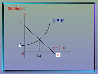
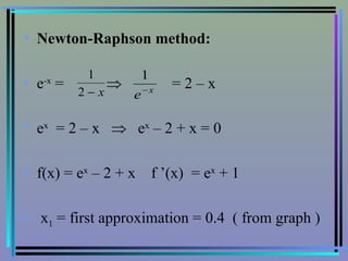
37. 0.4 - [ ] = = 0.4043 = 0.4043 - [ ] = 0.4433 = 0.4433 - [ ] = 0.4428 = 0.4428 - [ ] = 0.4428 The required solution is 0.443 ( three decimal places ).

38. EXERCISES 1.)By taking 0.2 as first approximation find the root of the equation ,giving your answer to three significant figures by using the Newton Raphson method. (Ans : 0.246)

39. 2.) Show that the equations 2sin x – x = 0 has a root between x = 1(radian) and x= 2 (radian). Find the root of the equation by using i) iteration method ii) Newton Raphson method Giving your answer to two decimal places.