Downloaded 91 times

![23
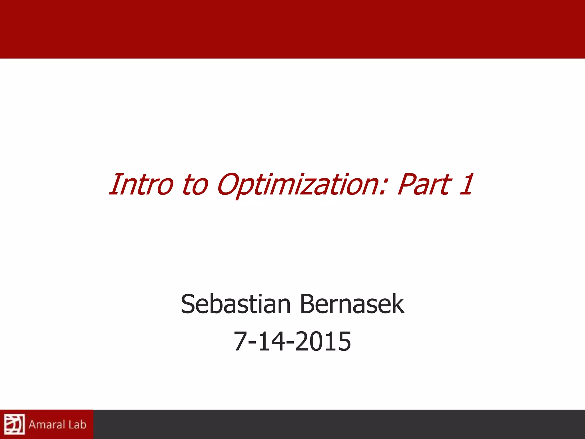
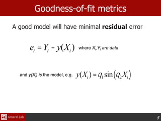
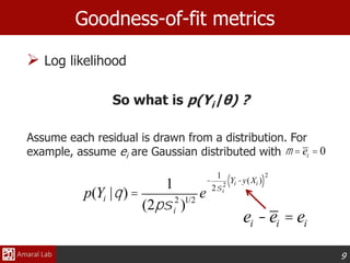
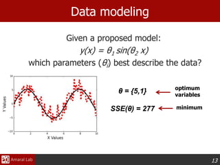
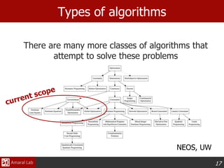
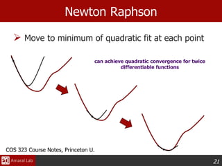
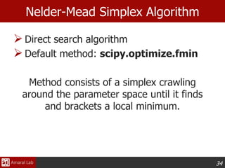
Newton’s Method in N-Dimensions
3. The minimum of the local second-order model
lies in the direction pn.
Determine the optimal step size, α, by 1-D optimization
pn = -H-1
(xn )Ñf (xn )
Search directionGeneral Iterative Scheme
α=step size
dn = search direction
xn+1 = xn +adn
a = argmina f (xn -aH-1
(xn )Ñf (xn ))éë ùû
a = argmina f (xn +apn )[ ]
Golden search,
Newton’s method,
Brent’s Method,
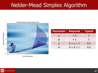
Nelder-Mead Simplex,
etc.](https://image.slidesharecdn.com/optimizationtutorial-150722170440-lva1-app6891/85/Optimization-tutorial-24-320.jpg)
![26
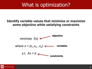
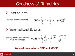
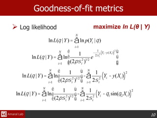
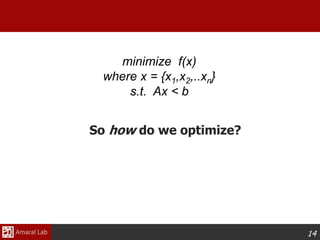
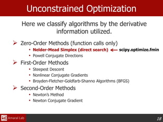
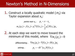
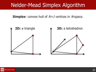
Gradient Descent
Newton/BFGS make use of the local Hessian
Alternatively we could just use the gradient
1. Pick a starting point, x0
2. Evaluate the local derivative
3. Perform line-search along gradient
1. Move directly along the gradient
2. Check convergence criteria and return to 2
Ñf (x0 )
xn+1 = xn -aÑf (xn )
a = argmina f (xn -aÑf (xn ))[ ]](https://image.slidesharecdn.com/optimizationtutorial-150722170440-lva1-app6891/85/Optimization-tutorial-27-320.jpg)
![27
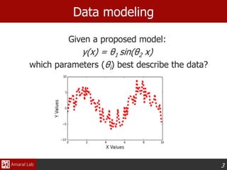
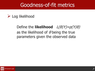
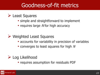
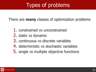
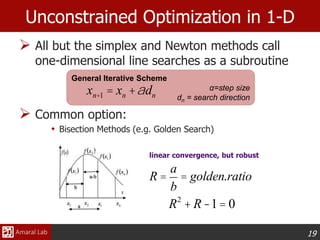
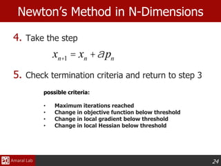
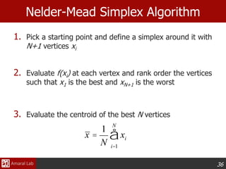
Gradient Descent
Function must be differentiable
Subsequent steps are always perpendicular
Can get caught in narrow valleys
xn+1 = xn -aÑf (xn )
a = argmina f (xn -aÑf (xn ))[ ]](https://image.slidesharecdn.com/optimizationtutorial-150722170440-lva1-app6891/85/Optimization-tutorial-28-320.jpg)
![28
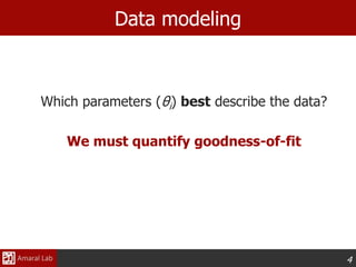
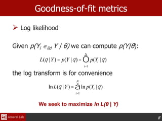
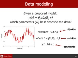
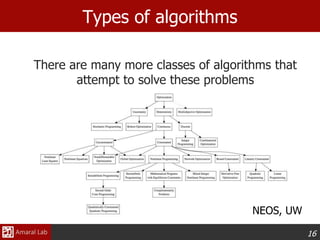
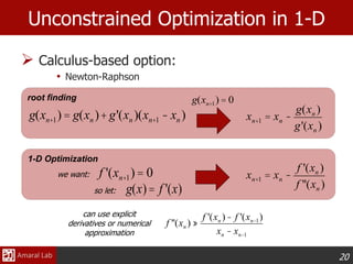
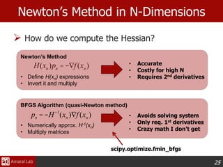
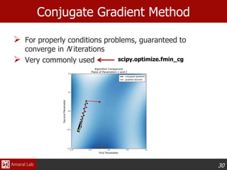
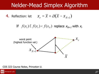
Conjugate Gradient Method
Avoids reversing previous iterations by ensuring that
each step is conjugate to all previous steps, creating a
linearly independent set of basis vectors
1. Pick a starting point and evaluate local derivative
2. First step follows gradient descent
3. Compute weights for previous steps, βn
x1 = x0 -aÑf (x0 )
a = argmina f (x0 -aÑf (x0 ))[ ]
bn =
Dxn
T
(Dxn -Dxn-1)
DxT
n-1Dxn-1
Dxn = -Ñf (xn )where
is the steepest direction
Polak-Ribiere Version](https://image.slidesharecdn.com/optimizationtutorial-150722170440-lva1-app6891/85/Optimization-tutorial-29-320.jpg)
![29
Conjugate Gradient Method
Creates a set, si, of linearly independent vectors
that span the parameter space xi.
4. Compute search direction, sn
4. Move to optimal point along sn
4. Check convergence criteria and return to step 3
xn+1 = xn +asn
a = argmina f (xn +asn )[ ]
*Note that setting βi = 0 yields the gradient descent algorithm
sn =-Ñf (xn )+bnsn-1](https://image.slidesharecdn.com/optimizationtutorial-150722170440-lva1-app6891/85/Optimization-tutorial-30-320.jpg)
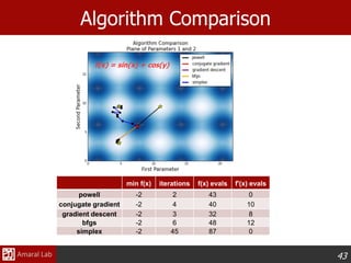
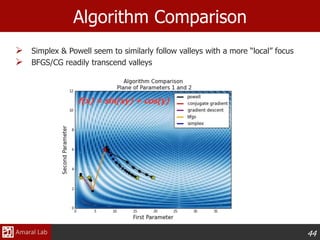
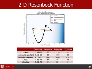

This document provides an overview of optimization techniques. It defines optimization as identifying variable values that minimize or maximize an objective function subject to constraints. It then discusses various applications of optimization in finance, engineering, and data modeling. The document outlines different types of optimization problems and algorithms. It provides examples of unconstrained optimization algorithms like gradient descent, conjugate gradient, Newton's method, and BFGS. It also discusses the Nelder-Mead simplex algorithm for constrained optimization and compares the performance of these algorithms on sample problems.