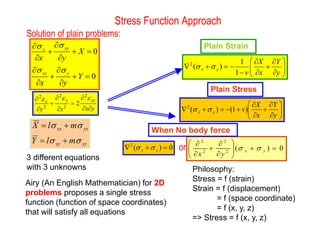
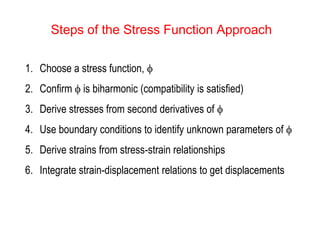
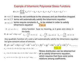
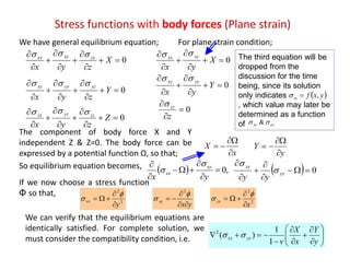
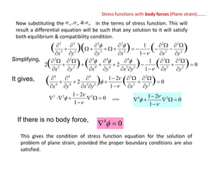
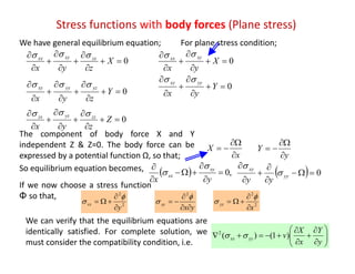
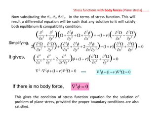
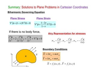
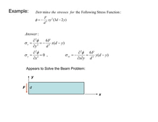
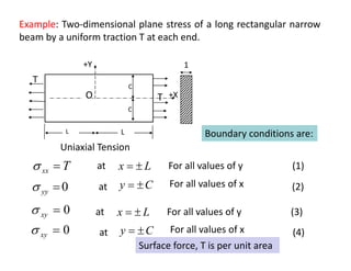
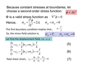
This document discusses the stress function approach for solving two-dimensional elasticity problems. It begins by presenting the general equations of elasticity, including stress-strain relationships, strain-displacement equations, and equilibrium equations. It then introduces the stress function method proposed by Airy, where a single function of space coordinates is assumed that satisfies all the elasticity equations. The key steps are: (1) choosing a stress function, (2) confirming it is biharmonic, (3) deriving stresses from its derivatives, (4) using boundary conditions to determine the function, (5) deriving strains, and (6) displacements. Examples of polynomial stress functions are also provided.

1. ME 6201: Applied Elasticity and Plasticity
STRESS FUNCTION
Cartesian coordinates
Prof. S.K.Sahoo

2. Plane
Stress
   
   
0,
1
1
1
,
1







yzxzxyxy
yxyxz
xyyyxx
E
E
EE










)(
2
1
0)(
2
1
)(
2
1
,,
x
w
z
u
y
w
z
xy
u
z
w
y
v
x
u
xz
yz
xy
zyx


































0 yzxzz 
Stress-strain
relationship
strain-displacement
equations
The equilibrium equations
Field equations
),(),,(),,( yxyxyx xyxyyyxx  
0
0












Y
yx
X
yx
yxy
xyx


Plane
Strain
0),,(),,(  wyxvvyxuu
0,2
)()(
2)(
2)(




yzxzxyxy
yxyxz
yyxy
xyxx
G
G
G




0
0












Y
yx
X
yx
yxy
xyx


0
)(
2
1
,,













yzxzz
xy
yx
xy
u
yx
u





)21)(1(
21
2
1
3
3
2













E
G
KGK
 = Lamé’s constant
G = shear modulus
xyxy
xyy
yxx
E
v
v
v
E
v
v
v
E
v



)1(
)
1
(
1
)
1
(
1
2
2










0 yzxzz 
xyxy
xyy
yxx
v
E
v
v
E
v
v
E



)1(
)(
1
)(
1
2
2









3. Simplified Elasticity Formulations
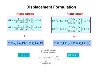
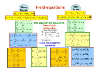
Displacement Formulation
Eliminate the stresses and strains
from the general system of
equations. This generates a system
of three equations for the three
unknown displacement components.
Equations are on u, v, w terms.
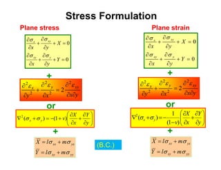
Stress Formulation
Eliminate the displacements and
strains from the general system of
equations. This generates a system
of six equations and for the six
unknown stress components.
Equations are on
terms
A practical elasticity problem may requires to solve 15 equations with 15
unknowns. It is very difficult to solve many real problems, so modified
formulations have been developed.
F(z)
G(x,y)
z
x
y Even using displacement or stress formulations
three-dimensional problems are difficult to solve.
So most solutions are assumed to of two-dimensional problems
],,,,,[ zxyzxyzzyyxx 

4. Displacement Formulation
0
)1(2
0
)1(2
2
2






























Y
y
v
x
u
yv
E
vG
X
y
v
x
u
xv
E
uG
Plane stress
+
),(),,( yxvvyxuu bb 
(B.C.)
Plane strain
+
),(),,( yxvvyxuu bb 
0)(
0)(
2
2




























Y
y
v
x
u
y
GvG
X
y
v
x
u
x
GuG


(B.C.)
)21)(1(
21
2
1
3
3
2













E
G
KGK
 = Lamé’s constant
G = shear modulus

5. Stress Formulation
yxxy
xyyx







 
2
2
2
2
2
2












y
Y
x
X
vyx )1()(2

0
0












Y
yx
X
yx
yxy
xyx


+
or
+
Plane stress Plane strain
0
0












Y
yx
X
yx
yxy
xyx















y
Y
x
X
v
yx
)1(
1
)(2

yyxy
yxxx
mlY
mlX




yyxy
yxxx
mlY
mlX




(B.C.)
or
yxxy
xyyx







 
2
2
2
2
2
2
+
+

6. Stress Function Approach
0
0












Y
yx
X
yx
yxy
xyx


yxxy
xyyx







 
2
2
2
2
2
2
Solution of plain problems:













y
Y
x
X
v
yx
1
1
)(2

Plain Strain












y
Y
x
X
vyx )1()(2

Plain Stress
0)(2
2
2
2











yx
yx

3 different equations
with 3 unknowns
Airy (An English Mathematician) for 2D
problems proposes a single stress
function (function of space coordinates)
that will satisfy all equations
yyxy
yxxx
mlY
mlX




When No body force
0)(2
 yx  or
Philosophy:
Stress = f (strain)
Strain = f (displacement)
= f (space coordinate)
= f (x, y, z)
=> Stress = f (x, y, z)

7. Airy Stress Function Method
Plane Problems with No Body Forces
0
0












yx
yx
yxy
xyx


0)(2
 yx
Stress Formulation
yxxy
xyyx















2
2
2
2
2
,,
Airy Representation
02 4
4
4
22
4
4
4









yyxx
Biharmonic Governing Equation
(Single Equation with Single function  satisfy equilibrium and
compatibility equations. The unknown parameters of stress function can
be find out by putting boundary conditions. )
0)(2
2
2
2











yx
yx

Let assume a stress function = (x,y)
such that:
or
Putting it on equilibrium equations, it
can be checked that both equations are
satisfied.
Putting on compatibility equation
gives

8. Steps of the Stress Function Approach
1. Choose a stress function, 
2. Confirm  is biharmonic (compatibility is satisfied)
3. Derive stresses from second derivatives of 
4. Use boundary conditions to identify unknown parameters of 
5. Derive strains from stress-strain relationships
6. Integrate strain-displacement relations to get displacements

9. Example of biharmonic Polynomial Stress Functions
 




2
0211
2
20011000
0 0
),( yAxyAxAyAxAAyxAyx
m n
nm
mn
terms do not contribute to the stresses and are therefore dropped1 nm
terms will automatically satisfy the biharmonic equation3 nm
terms require constants Amn to be related in order to satisfy
biharmonic equation
3 nm
cbyax ,If
22
If, cybxyax 
04
 
...........,If 2234222322
 ykxyjxhxgyfxyyexdxcybxyax
c
y
xx 2002
2





 0022
2



 a
x
yy

 00
2



 b
yx
xy


Stress distribution can be obtained but
all to satisfy biharmonic equation,
which requires that there exist some
relations among coefficients.
..........2006200200 2
kxgyfxcxx 
...........26120026002 22
kyjxyhxeydxayy 
..........430022000 2
kxyjxfyexbxy 
stress function have no meaning, as it gives zero stress in
the body.
Any quadratic function of x and y will automatically satisfy the biharmonic equation
but give constant values of stresses.
04
 

10. Stress functions with body forces (Plane strain)
0








X
zyx
zxxyxx 
0








Y
zyx
yzyyxy 
0








Z
zyx
zzyzzx 
0





X
yx
xyxx

0





Y
yx
yyxy 
0


z
zz
We have general equilibrium equation; For plane strain condition;
The component of body force X and Y
independent Z & Z=0. The body force can be
expressed by a potential function Ω, so that; x
X



y
Y



  ,0





yx
xy
xx

   0





yy
xy
yy

So equilibrium equation becomes,
2
2
y
xx





yx
xy





2
2
2
x
yy





If we now choose a stress function
Φ so that,
The third equation will be
dropped from the
discussion for the time
being, since its solution
only indicates
, which value may later be
determined as a function
of
 yxfzz ,
yyxx  &
We can verify that the equilibrium equations are
identically satisfied. For complete solution, we
must consider the compatibility condition, i.e. 












y
Y
x
X
v
yyxx
1
1
)(2


11. )())(( 2
2
2
2
2
2
2
2
2
2
2
2
1
1
yxxyyx 




















Stress functions with body forces (Plane strain)……..
xyyyxx  &,Now substituting the in the terms of stress function. This will
result a differential equation will be such that any solution to it will satisfy
both equilibrium & compatibility condition.
Simplifying,
It gives,
If there is no body force,
0
1
1
22 )()()( 2
2
2
2
22
4
4
4
4
4
2
2
2
2






















yxyxyxyx 

0
1
21
2 )()( 2
2
2
2
22
4
4
4
4
4

















yxyxyx 


0
1
21 222






 0
1
21 24







04
 
This gives the condition of stress function equation for the solution of
problem of plane strain, provided the proper boundary conditions are also
satisfied.

12. Stress functions with body forces (Plane stress)
0








X
zyx
zxxyxx 
0








Y
zyx
yzyyxy 
0








Z
zyx
zzyzzx 
0





X
yx
xyxx

0





Y
yx
yyxy 
We have general equilibrium equation; For plane stress condition;
The component of body force X and Y
independent Z & Z=0. The body force can be
expressed by a potential function Ω, so that; x
X



y
Y



  ,0





yx
xy
xx

   0





yy
xy
yy

So equilibrium equation becomes,
2
2
y
xx





yx
xy





2
2
2
x
yy





If we now choose a stress function
Φ so that,
We can verify that the equilibrium equations are
identically satisfied. For complete solution, we
must consider the compatibility condition, i.e. 











y
Y
x
X
vyyxx )1()(2


13. )())(( 2
2
2
2
2
2
2
2
2
2
2
2
)1(
yxxyyx 


















Stress functions with body forces (Plane stress)……..
xyyyxx  &,Now substituting the in the terms of stress function. This will
result a differential equation will be such that any solution to it will satisfy
both equilibrium & compatibility condition.
Simplifying,
It gives,
If there is no body force,
0)1(22 )()()( 2
2
2
2
22
4
4
4
4
4
2
2
2
2





















yxyxyxyx


0)1(2 )()( 2
2
2
2
22
4
4
4
4
4















yxyxyx

0)1( 222
  0)1( 24
 
04
 
This gives the condition of stress function equation for the solution of
problem of plane stress, provided the proper boundary conditions are also
satisfied.

14. Summary: Solutions to Plane Problems in Cartesian Coordinates
yxxy
xyyyxx















2
2
2
2
2
,,
Airy Representation for stresses
02 4
4
4
22
4
4
4









yyxx
Biharmonic Governing Equation
),(,),( yxfYyxfX yx 
Boundary Conditions
R
S
x
y
0)1( 24
  0
1
21 24







If there is no body force,
Plane Stress Plane Strain
yyxy
yxxx
mlY
mlX





15. Example:
)23(
:FunctionStressFollowingthemin
2
3
ydxy
d
F
forstressestheeDetr

Appears to Solve the Beam Problem:
x
y
dF
)(
6
,0
)(
6
:
3
2
2
2
32
2
ydy
d
F
yxx
ydx
d
F
y
Answer
xyy
x


















16. T
1
T
+X
+Y
L L
C
C
O
Uniaxial Tension
Example: Two-dimensional plane stress of a long rectangular narrow
beam by a uniform traction T at each end.
Boundary conditions are:
0yy
Txx 
0xy
Cy 
at (3)
at (2)
For all values of yLx 
For all values of x
0xy Cy at (4)For all values of x
at (1)For all values of yLx 
Surface force, T is per unit area

17. Because constant stresses at boundaries, let
choose a second-order stress function: 2
Ay
Φ is a valid stress function as 04
 
Hence, 0,22
2



 xyyyxx A
y



The first boundary condition implies that , 2
T
A 
So, the stress field solution is, 0,  xyyyxx T 
Let find the displacement field, i.e., u ,v
 
E
T
Ex
u
yyxxxx 



1
 
E
T
Ey
xxyyyy  

 1v
0
v







Gxy
u xy
xy

Total shear strain,
(5)
(6)
(7)

18. Integrating Equations (5) and (6) w.r.t. x & y
)(yfx
E
T
u 
)(v xgy
E
T
 
f(y) is a arbitrary function of y
g(x) is a arbitrary function of x
Putting in equation (7) cxgyfxgyf  )()(0)()( ''''
Integrating,
Dcyyf )( Dcxxg )( c, D are arbitrary constants
It gives, Dcyx
E
T
u  Dcxy
E
T
 v
Displacement boundary conditions are,
At x=0, y=0 u=0 & v=0 also v=0 at x=±L for all y
It gives, c=0 & D=0 So, final displacement field is,
x
E
T
u  y
E
T
v

19. 22
ByAx 
3
Ax  224
3 yxxA 
Problems: Prove that the followings are Airy’s stress function & examine the stress
distribution represented by them: , ,
22
ByAx 
,2Ax
x


 By
y
2


A
x
22
2


 B
y
22
2


 
04
4



x

04
4



y

022
4



yx

00002 4
4
22
4
4
4
4










yyxx


0,2,2
2
2
2
2
2










yx
A
x
B
y
xyyyxx






Ans:
Hence it is a Airy’s stress function.
It is a uniform two-dimensional stress function.
,3 2
Ax
x



04
4
2
2









yyy

Ax
x
62
2


 
A
x
63
3


 
04
4



x

04
  0,2,0  xyyxx Ax  One-dimensional linear stress field.
b) 022
4



yx

 23
64 xyxA
x



  yAxyxA
y
22
66 


 2
2
2
612 yxA
x


 
  22
2
2
66 AxxA
y


  Ax
x
243
3


 
04
4



y

A
x
244
4


 
Axy
yx
12
2


 
Ay
yx
122
3


 
A
yx
1222
4


 
0024244
 AA
2
6Axxx 
 22
612 yxAyy  Axyxy 12
,
,
So it is a Airy’s stress function, and
c)