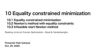
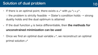
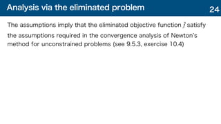
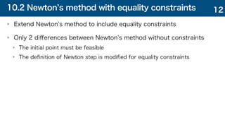
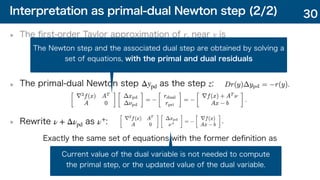
The document summarizes key points about equality constrained minimization problems and Newton's method for solving them. It discusses: 1) Equality constrained minimization problems and their equivalent forms via eliminating constraints or using the dual problem. 2) Newton's method extended to include equality constraints, where the Newton step is defined to satisfy the linearized optimality conditions and ensures feasible descent. 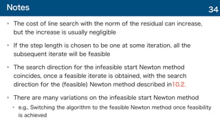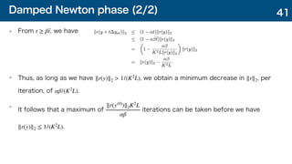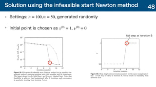3) An infeasible start Newton method that computes steps to reduce the primal-dual residual norm, ensuring iterates become feasible within a finite number of steps.

1. Presenter Koki Isokawa
Oct. 29, 2020
10 Equality constrained minimization
10.1 Equality constrained minimization
10.2 Newton s method with equality constraints
10.3 Infeasible start Newton method
Reading circle on Convex Optimization - Boyd & Vandenberghe

2. 10.1 Equality constrained minimization problems

3. Equality constrained minimization problem
Problem setting:
We assume the problem is solvable with optimal solution and
optimal value ,
minimize f(x) subject to Ax = b,
x⋆
p⋆
p⋆
= inf {f(x)|Ax = b} = f(x⋆
)
3
where is convex and twice continuously differentiable,
and with
f : Rn
→ R
A ∈ Rp×n
rank A = p < n . there are fewer constraints than variables
the equality constraints are independent

4. Equivalent problem
is optimal iff. there is a such that
Overview of this chapter
10.1.1: Introduce a simple problem
10.1.2: General solution via eliminating equality constraint
10.1.3: General solution via the dual
x⋆
ν⋆
∈ Rp
4
Review 5.5.3(KKT condition)
primal feasible equations
(linear)
dual feasible equations
(nonlinear)

5. 10.1.1 Equality constrained convex quadratic minimization
The special case of equality constrained minimization problem with
is quadratic
Equivalent problem:
Rewritten as :
linear equations in the variables
f
KKT system
n + p n + p x⋆
, ν⋆
5
where and
P ∈ Sn
+ A ∈ Rp×n
KKT matrix

6. Solution of KKT system
When KKT matrix is nonsingular, there is a unique optimal primal-
dual pair
When KKT matrix is singular, but the KKT system is solvable, any
solution yields an optimal pair
If the KKT system is not solvable, the quadratic opt. problem is
unbounded below or infeasible
(x⋆
, ν⋆
)
(x⋆
, ν⋆
)
6

7. Nonsingularity of the KKT matrix
Conditions equivalent to nonsingularity of the KKT matrix
where is a matrix for which
(See exercise 10.1)
𝒩(P) ∩ 𝒩(A) = {0}
Ax = 0, x ≠ 0 ⇒ xT
Px > 0
FT
PF ≻ 0, F ∈ Rn×(n−p)
ℛ(F) = 𝒩(A)
7

8. 10.1.2 Eliminating equality constraints
A general approach to solving the equality constrained problem
We can solve the resulting unconstrained problem
1. Choose a matrix and vector that parametrize the
feasible set:
is a particular solution of
2. Solve eliminated optimization problem:
3. Find the solution:
F ∈ Rn×(n−p) ̂
x ∈ Rn
̂
x Ax = b
ℛ(F) = 𝒩(A)
z ∈ Rn−p
x⋆
= Fz⋆
+ ̂
x .
8
(Review of 4.2.4)

9. 10.1.3 Solving equality constraint problems via the dual
Another approach to solving the equality constrained problem
The dual function (Review of 5.5.5):
The dual problem:
9
conjugate function (3.3)
f*(y) := supx∈dom(yT
x − f(x))

10. Solution of dual problem
If there is an optimal point, there exists a with
the problem is strictly feasible → Slater s condition holds → strong
duality holds and the dual optimum is attained
If the dual function is twice differentiable, then the methods for
unconstrained minimization can be used
Once we find an optimal dual variable , we reconstruct an optimal
primal solution
ν⋆
g(ν⋆
) = p⋆
.
g
ν⋆
x⋆
10

11. 10.2 Newton s method with equality constraints

12. 10.2 Newton s method with equality constraints
Extend Newton s method to include equality constraints
Only 2 differences between Newton s method without constraints
The initial point must be feasible
The definition of Newton step is modified for equality constraints
12

13. 10.2.1 The Newton step Δxnt
Definition via second-order approximation
Solution of linearized optimality conditions
The Newton decrement
Feasible descent direction
Affine invariance
13

14. Definition via second-order approximation
Minimize second-order Taylor approximation near with variable
(the optimal is )
This is a quadratic minimization problem with equality constraints,
and can be solved analytically (see 10.1.1)
x v
v Δxnt
14

15. Solution of linearized optimality conditions
Substitution:
Linearized approximation for the second equation
Using
x⋆
→ x + Δxnt, ν⋆
→ w
Ax = b,
15
Precisely coincide with the former definition

16. The Newton decrement
The Newton decrement (Preview of 9.5.1)
is the norm of the Newton step, in the norm defined by the Hessian
The difference between and the minimum of the second-order
model
λ
f(x)
̂
f(x + v)
16
(exercise 10.6)
• gives an estimate of , based on the quadratic model at
• or serves as the basis of a good stopping criterion
λ(x)2
/2 f(x) − p⋆
x
λ(x) λ(x)2

17. Feasible descent direction
Suppose
is called as a if
Every point is also feasible, i.e.,
is called as a for at , if for small
The Newton step is always a feasible descent direction
shows a feasible direction
shows a descent direction
Ax = b
v ∈ Rn
feasible direction Av = 0
x + tv A(x + tv) = b
v descent direction f x t > 0, f(x + tv) < f(x)
AΔxnt = 0
17

18. Affine invariance
The Newton step and decrement for equality constrained opt. are
affine invariant as well as those for unconstrained opt.
Let is nonsingular and define . Then we have
and the equality constraint becomes .
The Newton step for at is given by
Hence .
T ∈ Rn×n ¯
f(y) = f(Ty)
Ax = b ATy = b
¯
f y
TΔynt = Δxnt
18

19. 10.2.2 Newton s method with equality constraints
The outline is exactly the same as for unconstrained problems
The method is called a feasible descent method
19

20. 10.2.3 Newton s method and elimination (1/3)
The Newton s method for equality constrained problem coincide with
the Newton s method for reduced problem:
Both conditions for having the Newton step are equivalent
The Newton step for the reduced problem is defined, i.e., the hessian of the
reduced problem is invertible.
The Newton step for the equality constrained problem is defined, i.e., the
KKT matrix is invertible.
minimize ̂
f(z) = f(Fz + ̂
x)
∇2 ̂
f(x) = FT
∇2
f(Fz + ̂
x)F
[
∇2
f(x) AT
A 0 ]
20

21. 10.2.3 Newton s method and elimination (2/3)
Both search directions are precisely the same
The Newton step for the reduced problem :
The equations defining the Newton step for the equality constrained
problem: is hold by taking
and choosing
The second equation holds:
Equation as following holds:
Δznt
∇2
f(x)Δxnt + AT
w + ∇f(x) = 0, AΔxnt = 0 Δxnt = FΔznt
w = − (AAT
)−1
A(∇f(x) + ∇2
f(x)Δxnt)
AΔxnt = AFznt = 0 AF = 0
21
nonsingular
the first equation holds

22. 10.2.3 Newton s method and elimination (3/3)
Both Newton decrement are equal
22

23. 10.2.4 Convergence analysis
Everything about the convergence of Newton s method for
unconstrained problems transfers to Newton s method with equality
constrained
Assumptions:
The sublevel set is closed, where
satisfies
On the set , we have , and
i.e., the inverse of the KKT matrix is bounded on
For satisfies the Lipschitz condition
S = {x|x ∈ dom f, f(x) ≤ f(x(0)
), Ax = b}
x(0)
∈ dom f Ax(0)
= b
S ∇2
f(x) ⪯ MI
S
x, x̃ ∈ S, ∇2
f ∥∇2
f(x) − ∇2
f(x̃)∥2 ≤ L∥x − x̃∥2
23

24. Analysis via the eliminated problem
The assumptions imply that the eliminated objective function satisfy
the assumptions required in the convergence analysis of Newton s
method for unconstrained problems (see 9.5.3, exercise 10.4)
˜
f
24

25. 10.3 Infeasible start Newton method

26. 10.3 Infeasible start Newton method
Newton s method in 10.2 is a feasible descent method
Here, we describe a generalization of the method that works with
initial points, and iterates, that are not feasible
26

27. 10.3.1 Newton step at infeasible points
Optimality conditions:
Let denote the current point, which is not feasible, but
The goal is to find a step so that satisfies the optimality
conditions, i.e.,
We substitute for and for , and use the first-order
approximation:
x x ∈ dom f
Δx x + Δx
x + Δx ≃ x⋆
x + Δx x⋆
w ν⋆
27
When is feasible ( ),
the step coincides with the standard Newton step
x Ax − b = 0
Δx

28. Interpretation as primal-dual Newton step (1/2)
Give an interpretation with a - for the equality
constrained problem
Primal-dual method: update both thee primal variable , and the dual
variable , in order to satisfy the optimality conditions
We define as , where
The optimality conditions:
primal dual method
x
ν
r : Rn
× Rp
→ Rn
× Rp
r(x, ν) = (rdual(x, ν), rpri(x, ν))
r(x⋆
, ν⋆
) = 0
28

29. The first-order Taylor approximation of , near is
The primal-dual Newton step as the step :
Rewrite as :
r y
Δypd z
ν + Δνpd ν+
29
where is the derivative of , evaluated at
Dr(y) ∈ R(n+p)×(n+p)
r y
Interpretation as primal-dual Newton step (2/2)
Exactly the same set of equations with the former definition as

30. The first-order Taylor approximation of , near is
The primal-dual Newton step as the step :
Rewrite as :
r y
Δypd z
ν + Δνpd ν+
30
where is the derivative of , evaluated at
Dr(y) ∈ R(n+p)×(n+p)
r y
Interpretation as primal-dual Newton step (2/2)
Exactly the same set of equations with the former definition as
The Newton step and the associated dual step are obtained by solving a
set of equations, with the primal and dual residuals
Current value of the dual variable is not needed to compute
the primal step, or the updated value of the dual variable.

31. Residual norm reduction property
The Newton direction at an infeasible point is not necessarily a
descent direction for , i.e.,
The primal-dual interpretation shows that the norm of the residual
decreases in the Newton direction, i.e.,
Taking the derivative of the square:
f
31
is not necessarily negative
We can use to measure the progress of the infeasible start Newton method
∥r∥2

32. Full step feasibility property
Analysis using residual with a step length
The residual of the next step :
The residual after step:
It implies
The primal residual at each step is in the direction of , and is scaled down at
each step
Once a full step ( ) is taken, all future iterates are primal feasible
t ∈ [0,1]
r+
pri
k
r(0)
t = 1
32

33. 10.3.2 Infeasible start Newton method
Differences between the Newton method with feasible start
The search directions include the extra correction terms on the primal residual
The line search is carried out using the norm of the residual, instead of the function
value
The algorithm terminates when primal feasibility has been achieved, and the norm of the
(dual) residual is small
f
33

34. Notes
The cost of line search with the norm of the residual can increase,
but the increase is usually negligible
If the step length is chosen to be one at some iteration, all the
subsequent iterate will be feasible
The search direction for the infeasible start Newton method
coincides, once a feasible iterate is obtained, with the search
direction for the (feasible) Newton method described in10.2.
There are many variations on the infeasible start Newton method
e.g., Switching the algorithm to the feasible Newton method once feasibility
is achieved
34

35. Using infeasible start Newton method to simplify initialization
When is not all of , finding a point in that satisfies
can itself be a challenge
The general and the best way when is complex will be
introduced in the next chapter (11.4)
When is simple, and known to contain a point satisfying ,
the infeasible start Newton method gives a simple alternative
dom f Rn
dom f Ax = b
dom f
dom f Ax = b
35

36. 10.3.3 Convergence analysis
Here, we show that
Once the norm of the residual is small enough, the algorithm takes full
steps, and convergence is subsequently quadratic (Quadratically
convergent phase)
The norm of the residual is reduced by at least a fixed amount in each
iteration before the region of quadratic convergence is reached (Damped
Newton phase)
36

37. Assumptions
We make the following assumptions
The sublevel set is closed.
If is closed, then is a closed function, and therefore this condition is satisfied
for any and any (exercise 10.7)
On the set , we have for some
For , satisfies the Lipschitz condition
f ∥r∥2
x(0)
∈ dom f ν(0)
∈ Rp
S K
(x, ν), (x̃, ν̃) ∈ S Dr
37

38. Comparison with standard Newton method (10.2.4)
The second and third assumption are essentially the same with those
of standard Newton method
The first assumption about sublevel set is more generalized by using
residuals
38

39. A basic inequality
Let with , and be the Newton step at
Define
If for all , we define
Otherwise, is the smallest positive value of such that
For ,
We can show the following
y = (x, ν) ∈ S ∥r(y)∥2 ≠ 0 Δynt = (Δxnt, Δνnt) y
tmax = inf{t > 0|y + tΔynt ∉ S}
y + tΔynt ∈ S t ≥ 0 tmax = ∞
tmax t ∥r(y + tΔynt)∥2 = ∥r(y(0)
)∥2
0 ≤ t ≤ tmax y + tΔynt ∈ S
39
for 0 ≤ t ≤ min{1,tmax}

40. Damped Newton phase (1/2)
When , one iteration of the infeasible start Newton method
reduces by at least a certain minimum amount
The righthand is quadratic in , and monotonically decreasing between and its
minimizer
We must have based on the proof by contradiction, therefore
The step length satisfies the line search exit condition, so that we have , where
is the step length chosen by the backtracking algorithm
∥r(y)∥2 > 1/(K2
L)
∥r∥2
t t = 0
t̄ =
1
K2L∥r(y)∥2
< 1
tmax > t̄
t̄ t ≥ βt̄ t
40
for 0 ≤ t ≤ min{1,tmax}

41. Damped Newton phase (2/2)
From , we have
Thus, as long as we have , we obtain a minimum decrease in , per
iteration, of .
It follows that a maximum of iterations can be taken before we have
.
t ≥ βt̄
∥r(y)∥2 > 1/(K2
L) ∥r∥2
αβ/(K2
L)
∥r(y(0)
)∥2K2
L
αβ
∥r(y)∥2 ≤ 1/(K2
L)
41

42. Quadratically convergent phase
Suppose
From the basic inequality
We must have based on the proof by contradiction. Therefore, a full
step will be taken for all future iterations
For , the basic inequality is written as
The residual steps after is written as
∥r(y)∥2 ≤ 1/(K2
L)
tmax > 1
t = 1
t = 1
k ∥r(y)∥2 ≤ 1/K2
L
42
for 0 ≤ t ≤ min{1,tmax}
where y+
= y + Δynt
It implies quadratic convergence of to zero
∥r(y)∥2

43. 10.3.4 Convex-concave games
An unconstrained (zero-sum, two-player) game on is defined by
its
Player 1 makes a payment to player 2 in
and : the choice of the value by player 1 and 2 respectively
The goal of player 1 is minimizing the payment, while that of player 2 is
maximizing it
The resulting payoff:
A. When player 1 makes the first choice:
B. When player 2 makes the first choice:
Inequality A B always holds
The difference between the two payoffs can be interpreted as the advantage afforded
the second player
Rp
× Rq
payoff function f : Rp+q
→ R
f(u, v)
u ∈ Rp
v ∈ Rq
≥
43

44. Solution of the game
is a of the game, or a - for the game,
if for all ,
When a solution exists, there is no advantage to making the second choice;
is the common value of both payoffs (exercise 3.14)
The game is called - if for each is a convex function of
, and for each is a concave function of
When is differentiable, a saddle-point for the game is characterized by
(u⋆
, v⋆
) solution saddle point
u, v f(u⋆
, v) ≤ f(u⋆
, v⋆
) ≤ f(u, v⋆
)
f(u⋆
, v⋆
)
convex concave v, f(u, v)
u u, f(u, v) v
f
∇f(u⋆
, v⋆
) = 0
44
i.e., player 2 maximize the earned payoff

45. Solution via infeasible start Newton method
We can use the infeasible start Newton method to solve a convex-
concave game with twice differentiable payoff function
We define the residual as and apply the
infeasible start Newton method
We can guarantee convergence provided has bounded
inverse, and satisfies a Lipschitz condition on the sublebel set
Dr = ∇2
f
45

46. 10.3.5 Examples
Show 3 examples
A simple example
An infeasible example
A convex-concave game
46

47. A simple example: the analytic center problem 47

48. Solution using the infeasible start Newton method
Settings: , generated randomly
Initial point is chosen as
n = 100,m = 50
x(0)
= 1, ν(0)
= 0
48
full step at iteration 8

49. An infeasible example
Consider the the same problem, for which does not intersect
Note that it is infeasible
dom f
49
No full step
The residuals do not converge to zero

50. A convex-concave game
Define the payoff function as
Generated randomly
Started at
u ∈ R100
, v ∈ R100
A, b, c
u(0)
= v(0)
= 0
50