02 basics i-handout

Basic Concepts in Optimization – Part I
Benoˆıt Chachuat <benoit@mcmaster.ca>
McMaster University
Department of Chemical Engineering
ChE 4G03: Optimization in Chemical Engineering
Benoˆıt Chachuat (McMaster University) Basic Concepts in Optimization – Part I 4G03 1 / 23
Outline
1 Local and Global Optima
2 Numerical Methods: Improving Search
3 Notions of Convexity
Local Optima
Neighborhood
The neighborhood Nδ(x◦) of a point x◦ consists of all nearby points; that
is, all points within a small distance δ > 0 of x◦:
Nδ(x◦
)
∆
= {x : x − x◦
< δ}
Local Optimum
A point x∗ is a [strict] local minimum for the function f : IRn
→ IR on the
set S if it is feasible (x∗ ∈ S) and if suﬃciently small neighborhoods
surrounding it contain no points that are both feasible and [strictly] lower
in objective value:
∃δ > 0 : f (x∗
) ≤ f (x), ∀x ∈ S ∩ Nδ(x∗
)
[ ∃δ > 0 : f (x∗
) < f (x), ∀x ∈ S ∩ Nδ(x∗
) {x∗
} ]
Illustration of a (Strict) Local Minimum, x∗
δ
S
xx
Nδ(x∗)
f (x)
x∗
f (x∗)
f (x∗) < f (x), ∀x ∈ S ∩ Nδ(x∗) {x∗}

Global Optima
Global Optimum
A point x∗ is a [strict] global minimum for the function f : IRn
→ IR on the
set S if it is feasible (x∗ ∈ S) and if no other feasible solution has [strictly]
lower objective value:
f (x∗
) ≤ f (x), ∀x ∈ S
[ f (x∗
) < f (x), ∀x ∈ S {x∗
} ]
Remarks:
1 Global minima are always local minima
2 Local minima may not be global minima
3 Analog definitions hold for local/global optima to maximize problems
Illustration of a (Strict) Global Minimum, x∗
f (x∗)
S
x
x∗
f (x∗) < f (x), ∀x ∈ S {x∗}
f (x)
Global vs. Local Optima
Class Exercise: Identify the various types of minima and maxima for f on
S
∆
= [xmin, xmax]
f (x)
xmin xmax
x1 x2 x3 x4 x5
How to Find Optima?
Review: Three Methods for Optimization
1 Graphical Solutions
Great display + see multiple optima
But impractical for nearly all practical problems
2 Analytical Solutions (e.g., Newton, Euler, etc.)
Exact solution + easy analysis for changes in (uncertain) parameters
But not possible for most practical problems
3 Numerical Solutions
The only practical method for complex models!
But only guarantees local optima + challenges in finding effects of
(uncertain) parameters

Numerical Optimization: The Dilemma!
Consider the optimization problem:
min
0≤x1,x2≤5
f (x1, x2)
∆
=
1
1 + (x1 − 1)2 + (x2 − 1)2
+
0.5
1 + (x1 − 4)2 + (x2 − 3)2
0
1
2
3
4
5 0
1
2
3
4
5
0
0.2
0.4
0.6
0.8
1
1.2
f (x1, x2)
x1 x2
Numerical Optimization: The Dilemma!
Typically, only some local information is know about the objective function
typically at a current point x◦ = (x◦
1 , x◦
2 )!
Question: Which move do I make next?
current point
0
1
2
3
4
5 0
1
2
3
4
5
0
0.2
0.4
0.6
0.8
1
1.2
f (x1, x2)
x1 x2
Numerical Optimization: The Basic Approach
Improving Search
Improving search methods are numerical algorithms that begin at a
feasible solution to a given optimization model, and advance along a
search path of feasible points with ever-improving function value
0
1
2
3
4
5 0
1
2
3
4
5
0
0.2
0.4
0.6
0.8
1
1.2
f (x1, x2)
x1 x2
Direction-Step Paradigm
At the current point x(k), how do I decide:
the direction of change
the magnitude of change
whether further improvement is possible?
The Basic Equation
Improving search advances from current point x(k) to new point x(k+1) as:
x(k+1)
=






x
(k+1)
1
x
(k+1)
2
...
x
(k+1)
n






= x(k)
+ α∆x =






x
(k)
1
x
(k)
2
...
x
(k)
n






+ α





∆x1
∆x2
...
∆xn





where:
∆x deﬁnes a move direction of solution change at x(k) ( ∆x = 1)
α > 0 determines a move magnitude, how far to pursue this direction

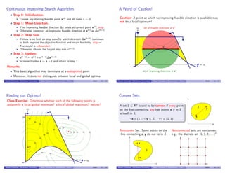
Direction of Change, ∆x
Improving Directions
Vector ∆x ∈ IRn
is an improving direction at current point x(k) if the
objective function value at x(k) + α∆x is superior to that of x(k), for all
α > 0 sufficiently small
(maximize problem) ∃¯α > 0 : f (x(k)
+ α∆x) > f (x(k)
), ∀α ∈ (0, ¯α]
0
1
2
3
4
5 0
1
2
3
4
5
0
0.2
0.4
0.6
0.8
1
1.2
f (x1, x2)
x1 x2
current point
∆x, improving direction
Direction of Change, ∆x
Improving Directions
Vector ∆x ∈ IRn
is an improving direction at current point x(k) if the
objective function value at x(k) + α∆x is superior to that of x(k), for all
α > 0 sufficiently small
(maximize problem) ∃¯α > 0 : f (x(k)
+ α∆x) > f (x(k)
), ∀α ∈ (0, ¯α]
x(k)
x(k+1)
x1
x2
set of improving directions at x(k)
set of improving directions at x(k+1)
Direction of Change, ∆x (cont’d)
Feasible Directions
Vector ∆x ∈ IRn
is an feasible direction at current point x(k) if point
x(k) + α∆x violates no model constraint for all α > 0 sufficiently small
∃¯α > 0 : x(k)
+ α∆x ∈ S, ∀α ∈ (0, ¯α]
x(k)
x1x1
x2
set of feasible directions at x(k)
Optimality Criterion
Necessary Condition of Optimality (NCO)
No optimization model solution at which an improving feasible direction is
available can be a local optimum
x∗
x1
x2
set of feasible directions at x∗
set of improving directions at x∗

Continuous Improving Search Algorithm
Step 0: Initialization.
◮ Choose any starting feasible point x(0)
and let index k ← 0.
Step 1: Move Direction.
◮ If no improving feasible direction ∆x exists at current point x(k)
, stop.
◮ Otherwise, construct an improving feasible direction at x(k)
as ∆x(k+1)
.
Step 2: Step Size.
◮ If there is no limit on step sizes for which direction ∆x(k+1)
continues
to both improve the objective function and retain feasibility, stop —
The model is unbounded.
◮ Otherwise, choose the largest step size α(k+1)
.
Step 3: Update.
◮ x(k+1)
← x(k)
+ α(k+1)
∆x(k+1)
◮ Increment index k ← k + 1 and return to step 1.
Remarks:
This basic algorithm may terminate at a suboptimal point
Moreover, it does not distinguish between local and global optima
A Word of Caution!
Caution: A point at which no improving feasible direction is available may
not be a local optimum!
x∗
x1
x2 set of feasible directions at x∗
set of improving directions at x∗
Finding out Optima!
Class Exercise: Determine whether each of the following points is
apparently a local/global minimum? a local/global maximum? neither?
10 20 30 40
30
40
20
60
40
50
50
50
60
90
60
70
100
70
80
x1
x2
Convex Sets
A set S ⊂ IRn
is said to be convex if every point
on the line connecting any two points x, y in S
is itself in S,
γx + (1 − γ)y ∈ S, ∀γ ∈ (0, 1)
x
yS
Nonconvex Set: Some points on the
line connecting x, y do not lie in S
S
x
y
Nonconnected sets are nonconvex;
e.g., the discrete set {0, 1, 2, . . .}2

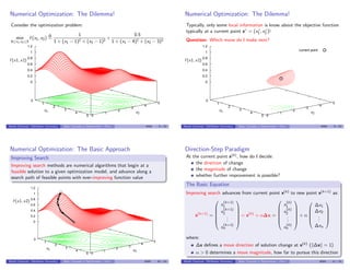
Convex and Concave Functions
Convex Functions
A function f : S → IR, defined on a convex set S ⊂ IRn
, is said to be
convex on S if the line segment connecting f (x) and f (y) at any two
points x, y ∈ S lies above the function between x and y,
f (γx + (1 − γ)y) ≤ γf (x) + (1 − γ)f (y), ∀γ ∈ (0, 1)
Strict convexity:
f (γx + (1 − γ)y) < γf (x) + (1 − γ)f (y), ∀x, y ∈ S, ∀γ ∈ (0, 1)
Concave Functions
f is said to be [strictly] concave on S if (−f ) is [strictly] convex on S,
f (γx + (1 − γ)y) ≥ [>]γf (x) + (1 − γ)f (y), ∀x, y ∈ S, ∀γ ∈ (0, 1)
Convex and Concave Functions (cont’d)
Case of a strictly convex function
on the convex set S
Case of a nonconvex function on S,
yet convex on the convex set S′
SS
S′
γx1 + (1 − γ)x2
f (γx1 + (1 − γ)x2)
γf (x1) + (1 − γ)f (x2)
x1 x1x2 x2
f (x)f (x)
Sets Defined by Constraints
Define the set S
∆
= {x ∈ IRn
: g(x) ≤ 0}, with g a
convex function on IRn
. Then, S is a convex set
Why?
g(x) = 0
S
Consider any two points x, y ∈ S. By the convexity of g,
g(γx + (1 − γ)y) ≤ γg(x) + (1 − γ)g(y), ∀γ ∈ (0, 1)
Since g(x) ≤ 0 and g(y) ≤ 0,
g(x) + (1 − γ)g(y) ≤ 0, ∀γ ∈ (0, 1)
Therefore, γx + (1 − γ)y ∈ S for every γ ∈ (0, 1); i.e., S is convex
Class Exercise: Give a condition on g for the following set to be convex:
S
∆
= {x ∈ IRn
: g(x) ≥ 0}
Sets Defined by Constraints (cont’d)
What is the condition on h for the following
set to be convex:
S
∆
= {x ∈ IRn
: h(x) = 0}
The set S is convex if and only if h is affine
x
y h(x) = 0
S
points not in S
Convex Sets Defined by Constraints
Consider the set
S
∆
= {x ∈ IRn
: g1(x) ≤ 0, . . . , gm(x) ≤ 0, h1(x) = 0, . . . , hp(x) = 0}
Then, S is convex if:
g1, . . . , gm are convex on IRn
h1, . . . , hp are affine

Convexity and Global Optimality
Consider the constrained program:
max
x
f (x)
s.t. gj (x) ≤ 0, j = 1, . . . , m
hj (x) = 0, j = 1, . . . , p
If f and g1, . . . , gm are convex on IRn
, and h1, . . . , hp are aﬃne, then
this program is said to be a convex program
Suﬃcient Condition for Global Optimality
A [strict] local minimum to a convex program is also a [strict] global
minimum
On the other hand, a nonconvex program may or may not have local
optima that are not global optima

02 basics i-handout

Recommended

Recommended

More Related Content

What's hot

What's hot (20)

Similar to 02 basics i-handout

Similar to 02 basics i-handout (20)

More from sheetslibrary

More from sheetslibrary (20)

Recently uploaded

Recently uploaded (20)

02 basics i-handout