


![SIMPSON’S
𝟏
𝟑
𝒓𝒅 RULE
𝑥0
𝑥1
𝑓(𝑥) 𝑑𝑥 =
ℎ
3
𝑦0 + 𝑦𝑛 + 4 𝑦1 + 𝑦3 + 𝑦5 + ⋯ + 2(𝑦2 + 𝑦4 + 𝑦6+. . )
=
ℎ
3
𝑓𝑖𝑟𝑠𝑡 + 𝑙𝑎𝑠𝑡 + 4 𝑠𝑢𝑚 𝑜𝑓 𝑜𝑑𝑑 𝑡𝑒𝑟𝑚𝑠 +
2 𝑠𝑢𝑚 𝑜𝑓 𝑒𝑣𝑒𝑛 𝑡𝑒𝑟𝑚𝑠 ]
ℎ =
𝑥1−𝑥0
𝑛
, 𝑛 − 𝑖𝑠 𝑡ℎ𝑒 𝒆𝒗𝒆𝒏 𝑛𝑜 𝑜𝑓 𝑠𝑢𝑏 𝑖𝑛𝑡𝑒𝑟𝑣𝑎𝑙𝑠 𝑖𝑛 𝑥0 𝑥1
Condition for applying the Simpson’s rule – Number
of subintervals must be even](https://image.slidesharecdn.com/interpolation-200303143708/75/Interpolation-22-2048.jpg)

![TRAPEZOIDAL RULE
𝑎
𝑏
𝑐
𝑑
𝑓 𝑥, 𝑦 𝑑𝑥𝑑𝑦 =
ℎ𝑘
4
𝑓1 + 𝑓3 + 𝑓7 + 𝑓9 +
2 𝑓2 + 𝑓4 + 𝑓6 + 𝑓8 + 4𝑓5]
=
ℎ𝑘
4
𝑆𝑢𝑚 𝑜𝑓 𝑐𝑜𝑟𝑛𝑒𝑟 𝑣𝑎𝑙𝑢𝑒𝑠 𝑜𝑓 𝑓 𝑥, 𝑦 +
2 𝑆𝑢𝑚 𝑜𝑓 𝑡ℎ𝑒 𝑏𝑜𝑢𝑛𝑑𝑎𝑟𝑦 𝑣𝑎𝑙𝑢𝑒𝑠 𝑜𝑓 𝑓 𝑥, 𝑦 +
4(𝑆𝑢𝑚 𝑜𝑓 𝑡ℎ𝑒 𝑖𝑛𝑡𝑒𝑟𝑖𝑜𝑟 𝑣𝑎𝑙𝑢𝑒𝑠 𝑜𝑓 𝑓(𝑥, 𝑦)]](https://image.slidesharecdn.com/interpolation-200303143708/75/Interpolation-24-2048.jpg)

![𝑺𝑰𝑴𝑷𝑺𝑶𝑵’𝑺 𝑹𝑼𝑳𝑬
𝑎
𝑏
𝑐
𝑑
𝑓 𝑥, 𝑦 𝑑𝑥𝑑𝑦 =
ℎ𝑘
9
𝑓1 + 𝑓3 + 𝑓7 + 𝑓9 +
2 𝑓2 + 𝑓4 + 𝑓6 + 𝑓8 + 16𝑓5]
=
ℎ𝑘
9
𝑆𝑢𝑚 𝑜𝑓 𝑐𝑜𝑟𝑛𝑒𝑟 𝑣𝑎𝑙𝑢𝑒𝑠 𝑜𝑓 𝑓 𝑥, 𝑦 +
4 𝑆𝑢𝑚 𝑜𝑓 𝑡ℎ𝑒 𝑏𝑜𝑢𝑛𝑑𝑎𝑟𝑦 𝑣𝑎𝑙𝑢𝑒𝑠 𝑜𝑓 𝑓 𝑥, 𝑦 +
16(𝑆𝑢𝑚 𝑜𝑓 𝑡ℎ𝑒 𝑖𝑛𝑡𝑒𝑟𝑖𝑜𝑟 𝑣𝑎𝑙𝑢𝑒𝑠 𝑜𝑓 𝑓(𝑥, 𝑦)]](https://image.slidesharecdn.com/interpolation-200303143708/75/Interpolation-26-2048.jpg)


This document discusses various methods of interpolation and numerical differentiation using divided differences and Newton's formulas. It introduces Lagrange interpolation for both equal and unequal intervals. Inverse interpolation and Newton's divided difference interpolation are also covered. Forward and backward difference formulas are presented for interpolation with equal intervals. Numerical differentiation can be performed by taking derivatives of the interpolation polynomial or using forward difference formulas to estimate derivatives at the data points.
Introduction to Interpolation, a method for estimating values between known data points.
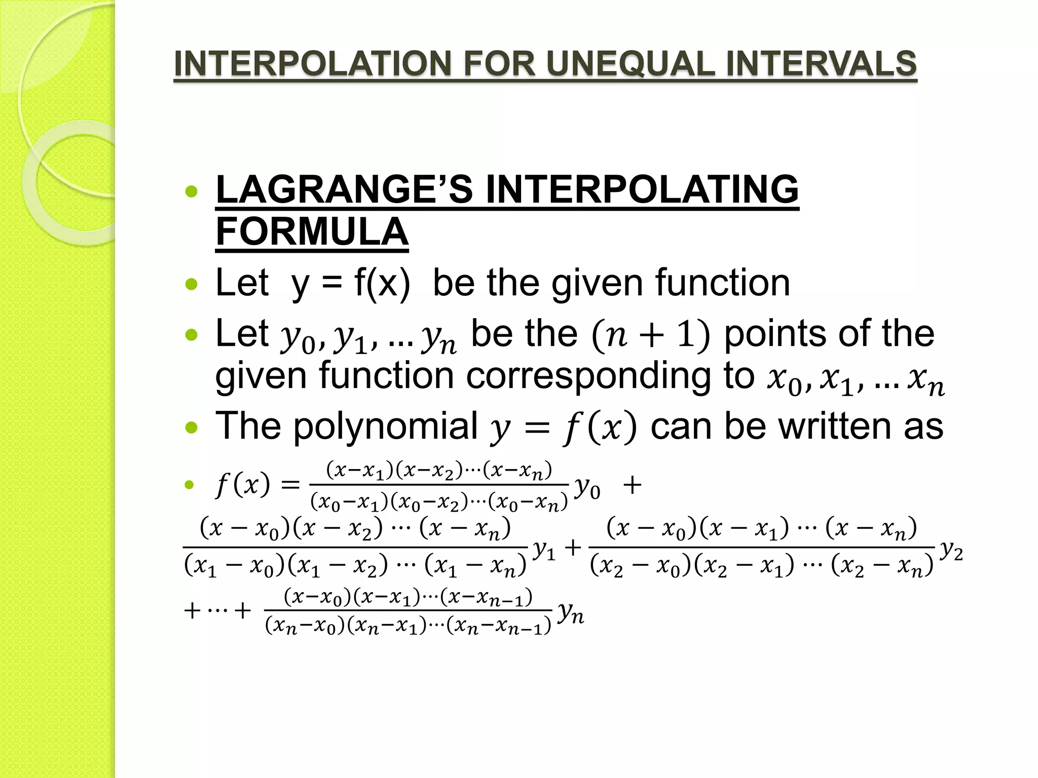
Details of Lagrange's interpolating formula for unequal intervals, derived from known values.
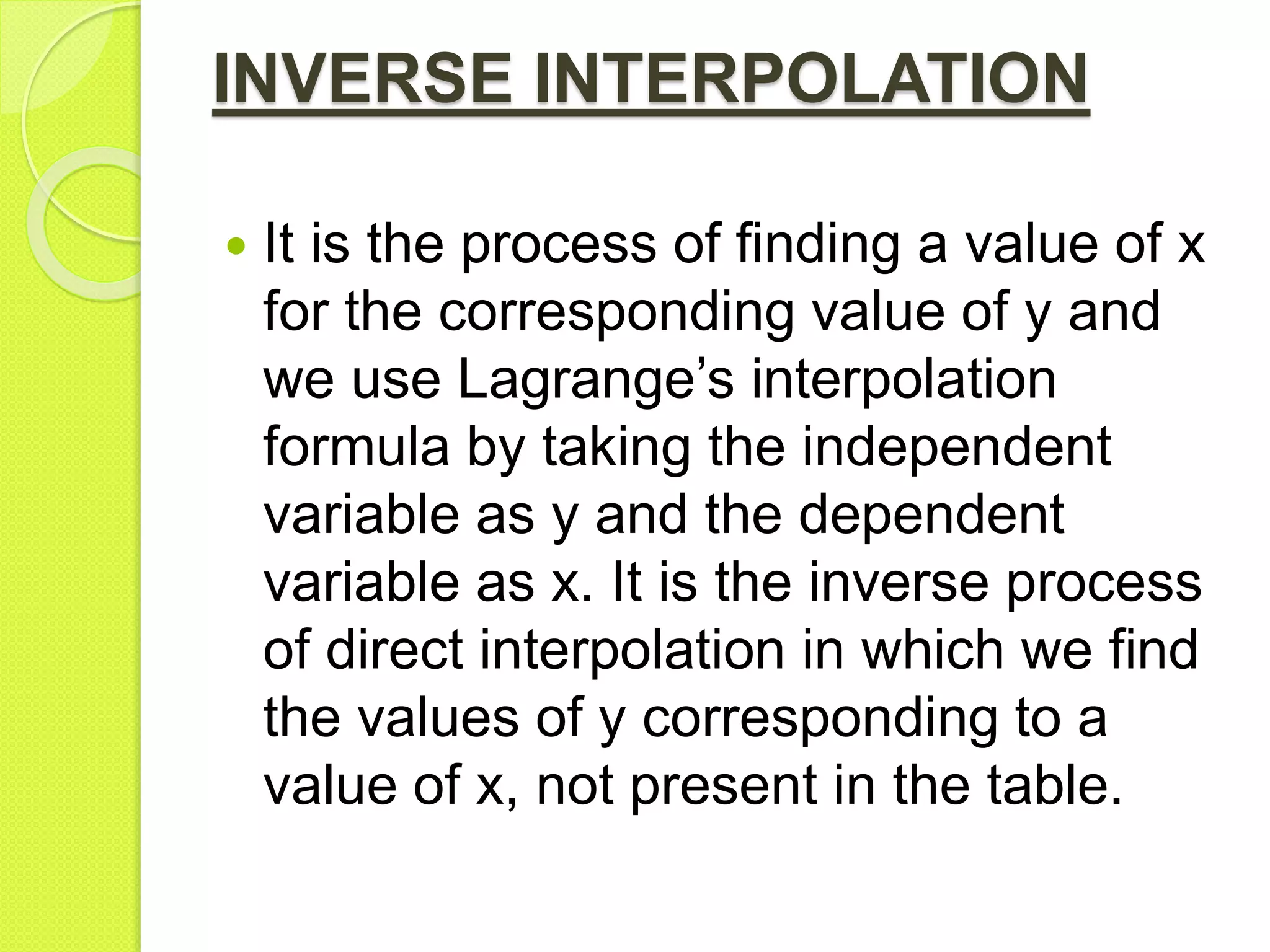
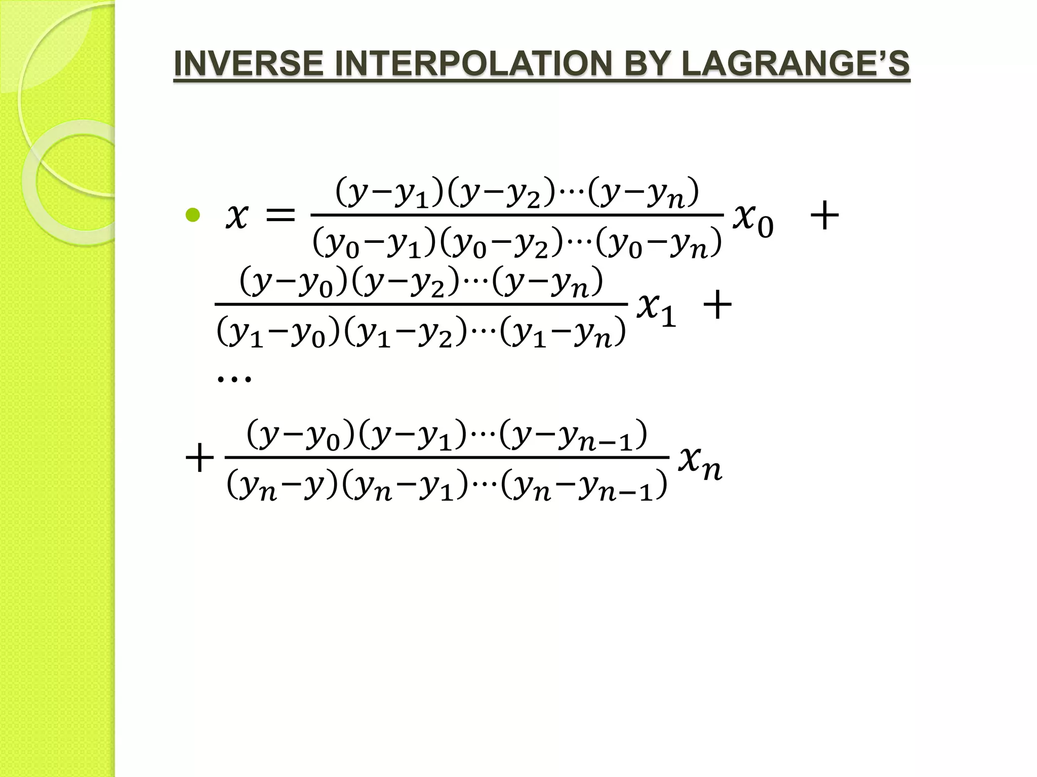
Explanation of inverse interpolation using Lagrange’s formula, to find x from known y values.
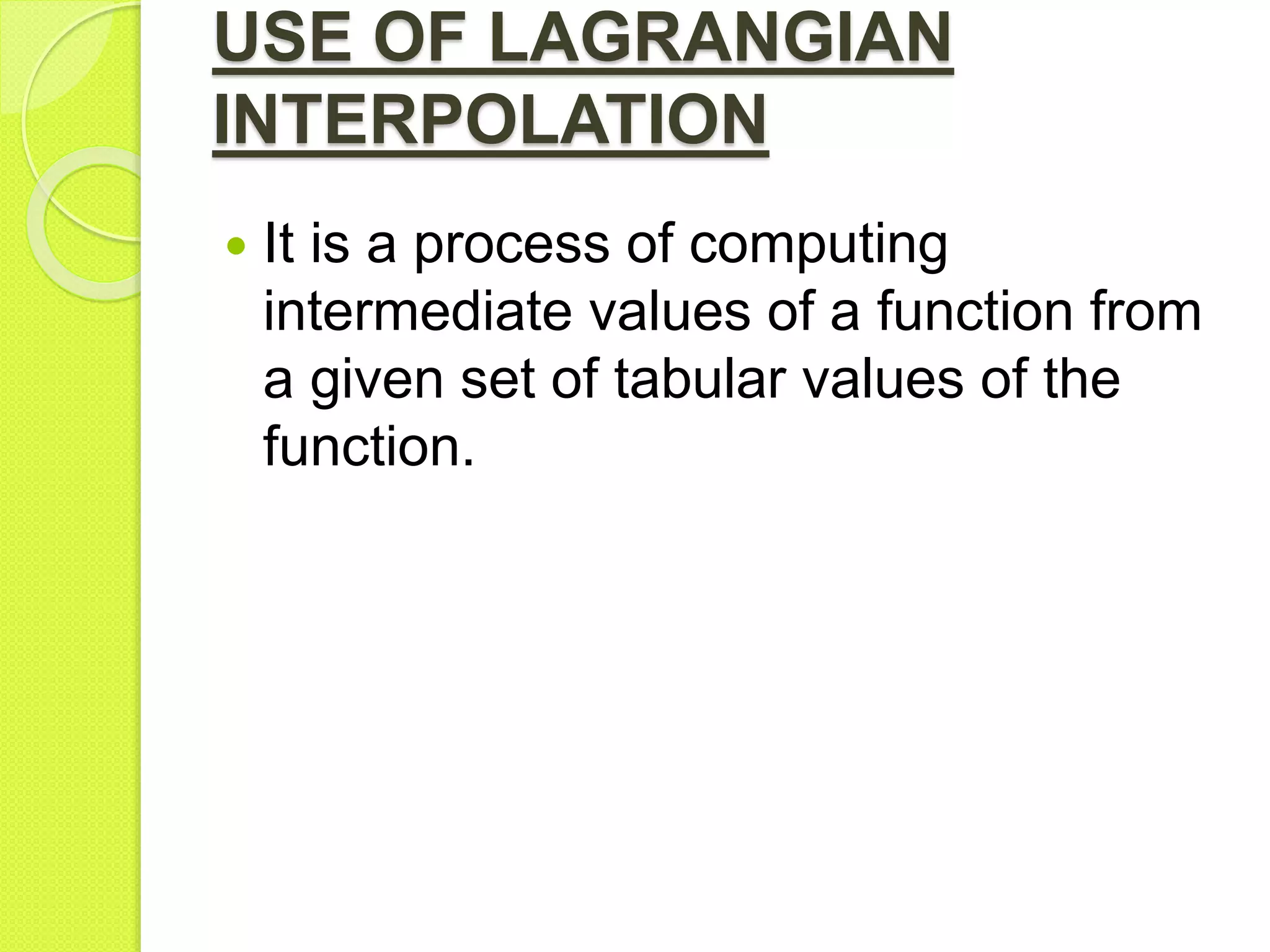
Describes the use of Lagrangian interpolation for computing intermediate values from tabulated data.
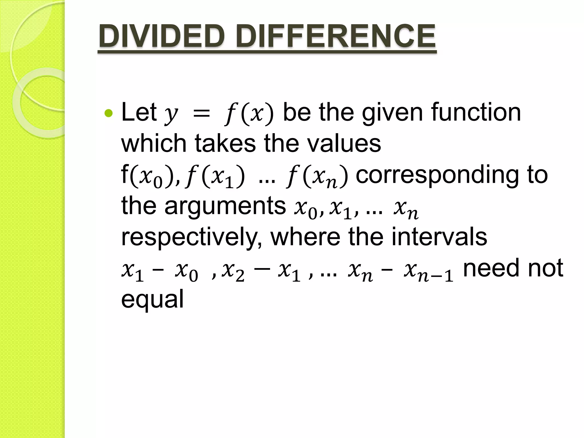
Introduction to divided differences for functions at specified intervals, regardless of equal spacing.
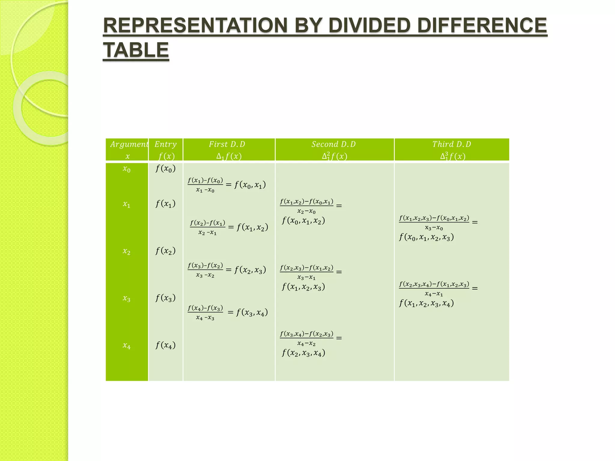
Representation and calculation of divided differences using a divided difference table.
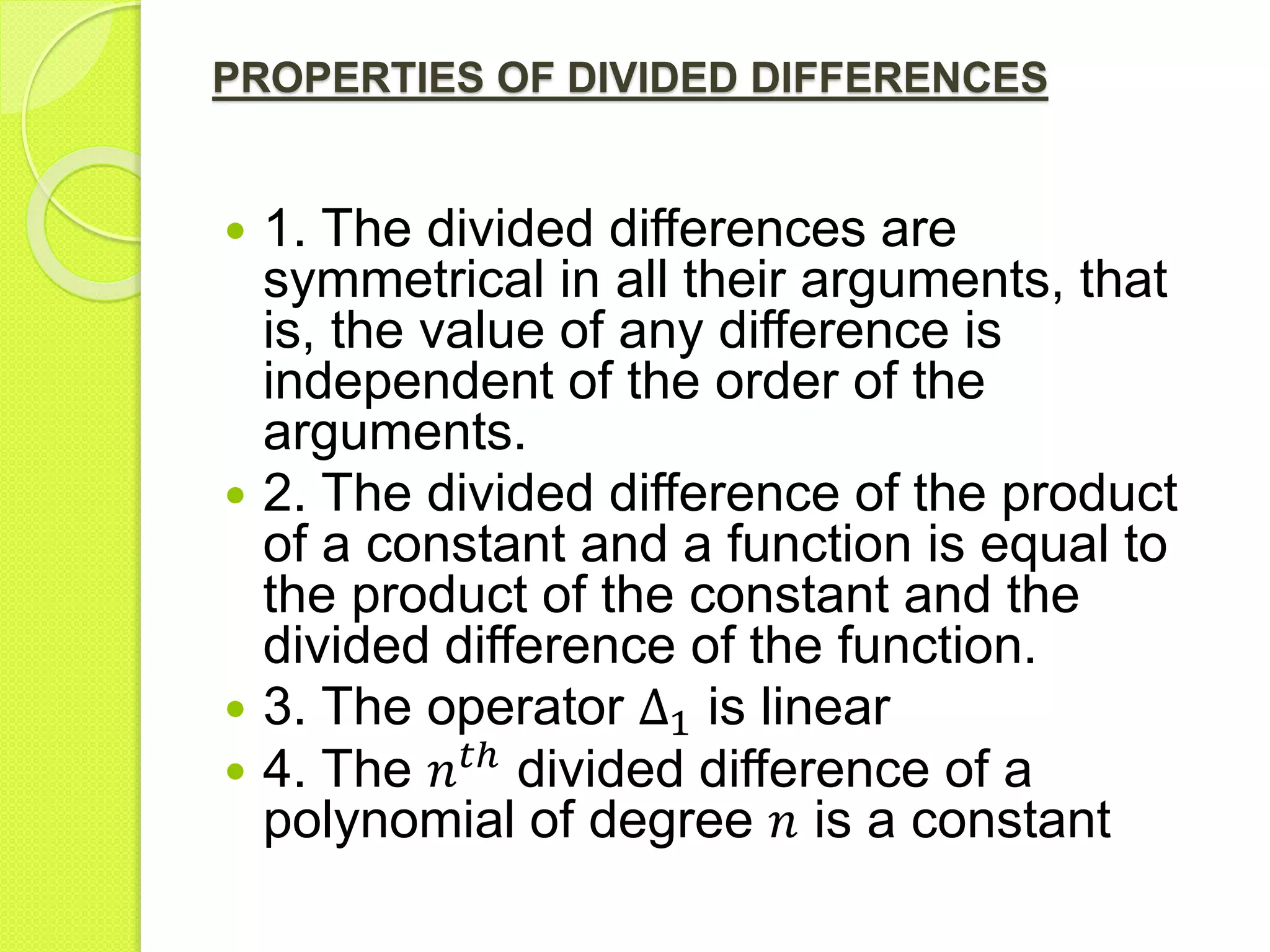
Key properties of divided differences, including symmetry, linearity, and characteristics of polynomial differences.
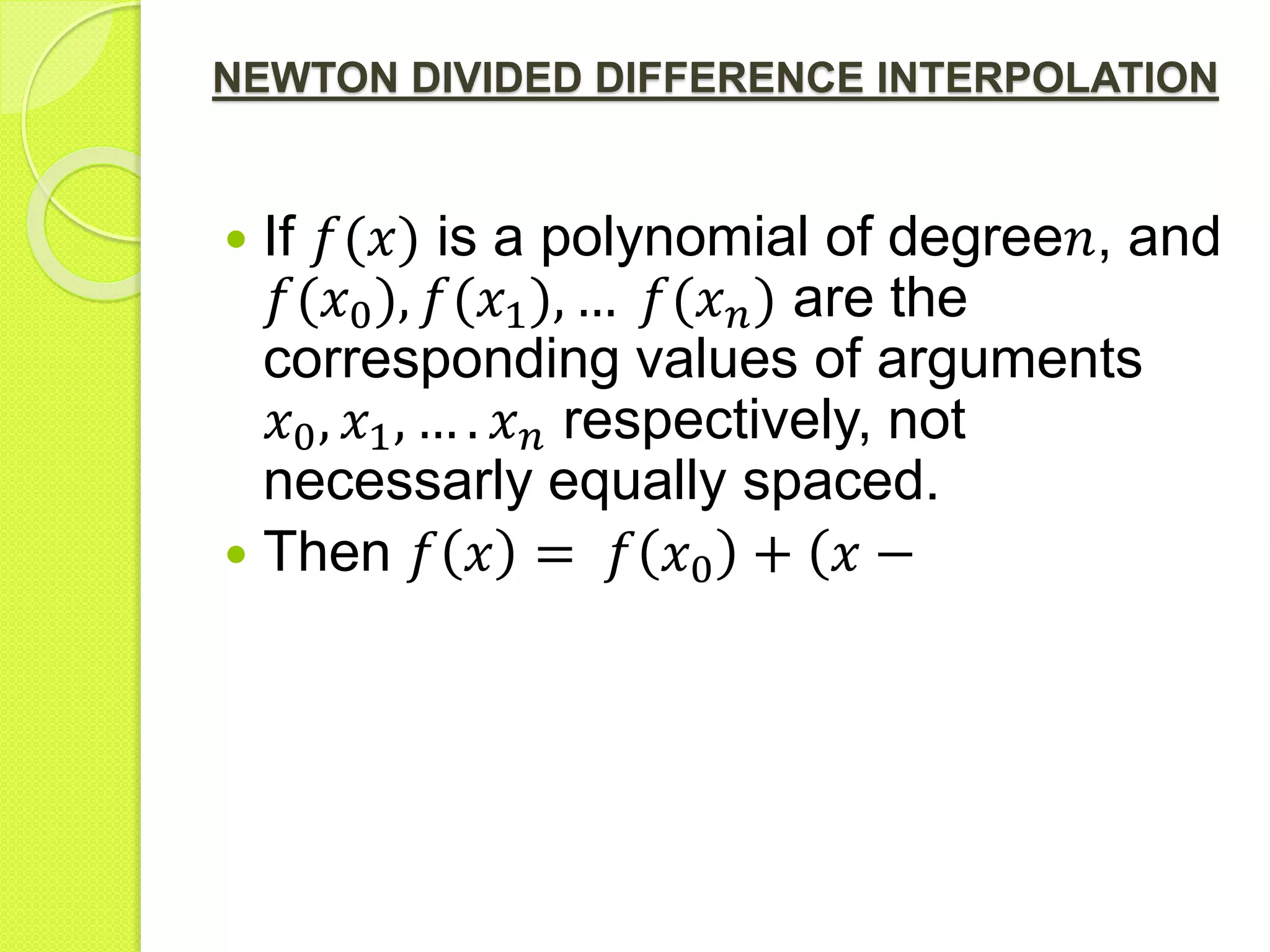
Method for interpolating polynomial functions using Newton's divided difference formula.
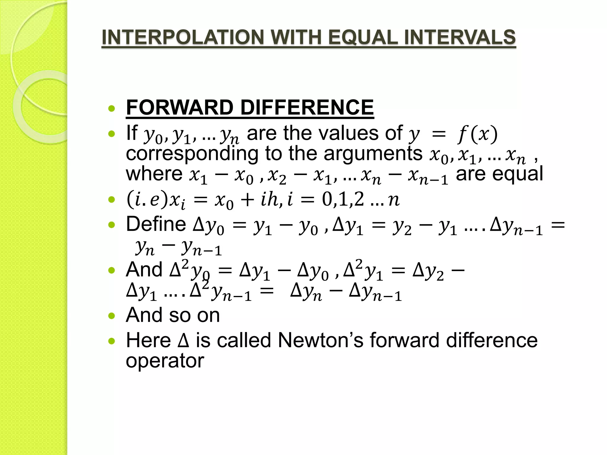
Describes forward differences for equal interval data sets for interpolation calculations.
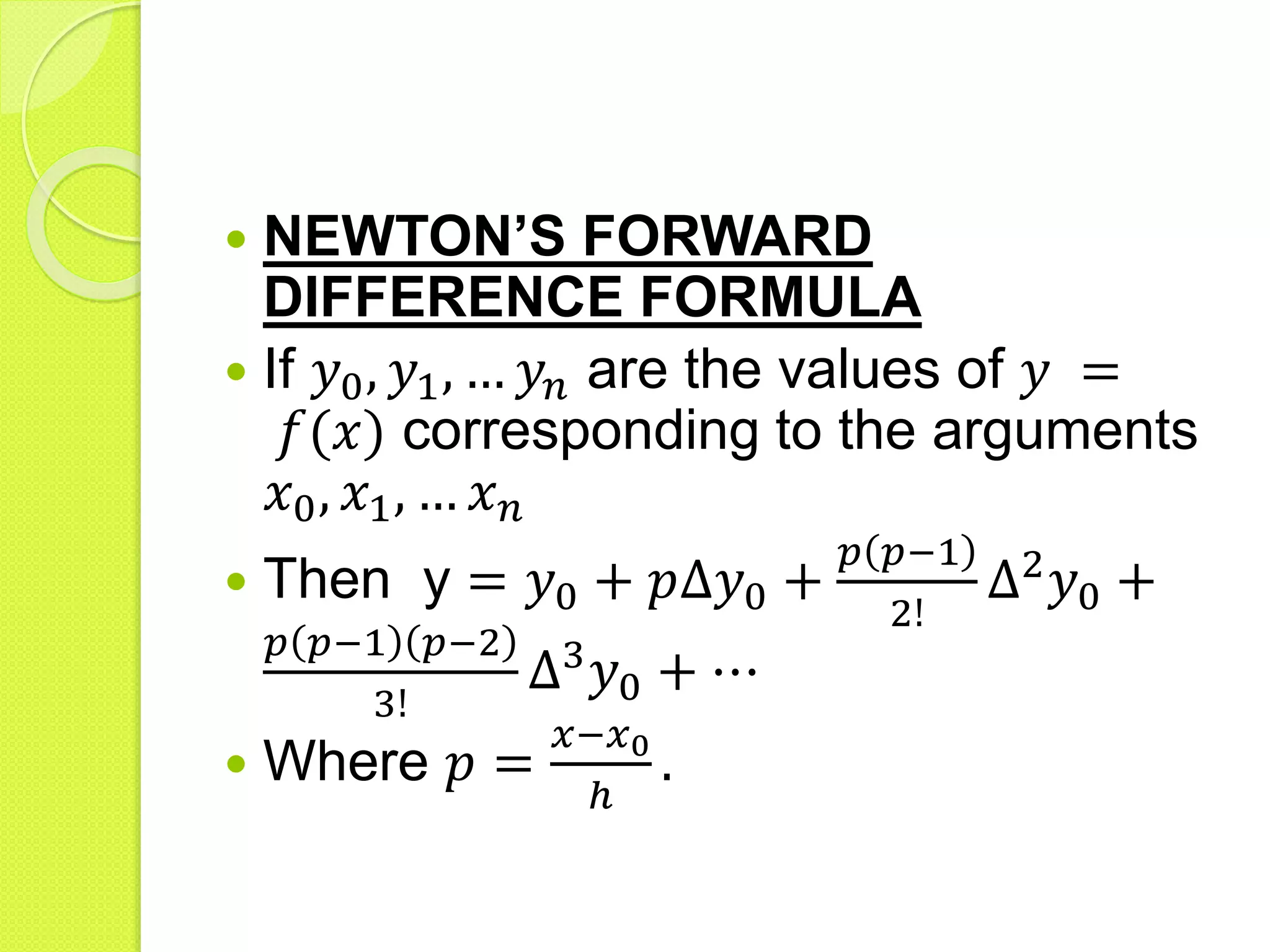
Formula for Newton’s forward differences for estimating function values at new points.
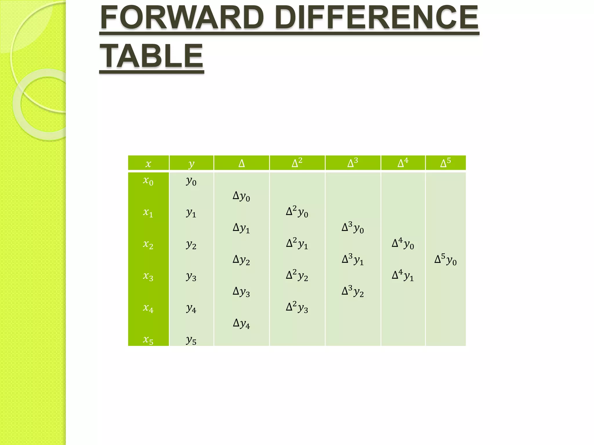
Table structure for organizing values and their differences for Newton’s forward difference method.
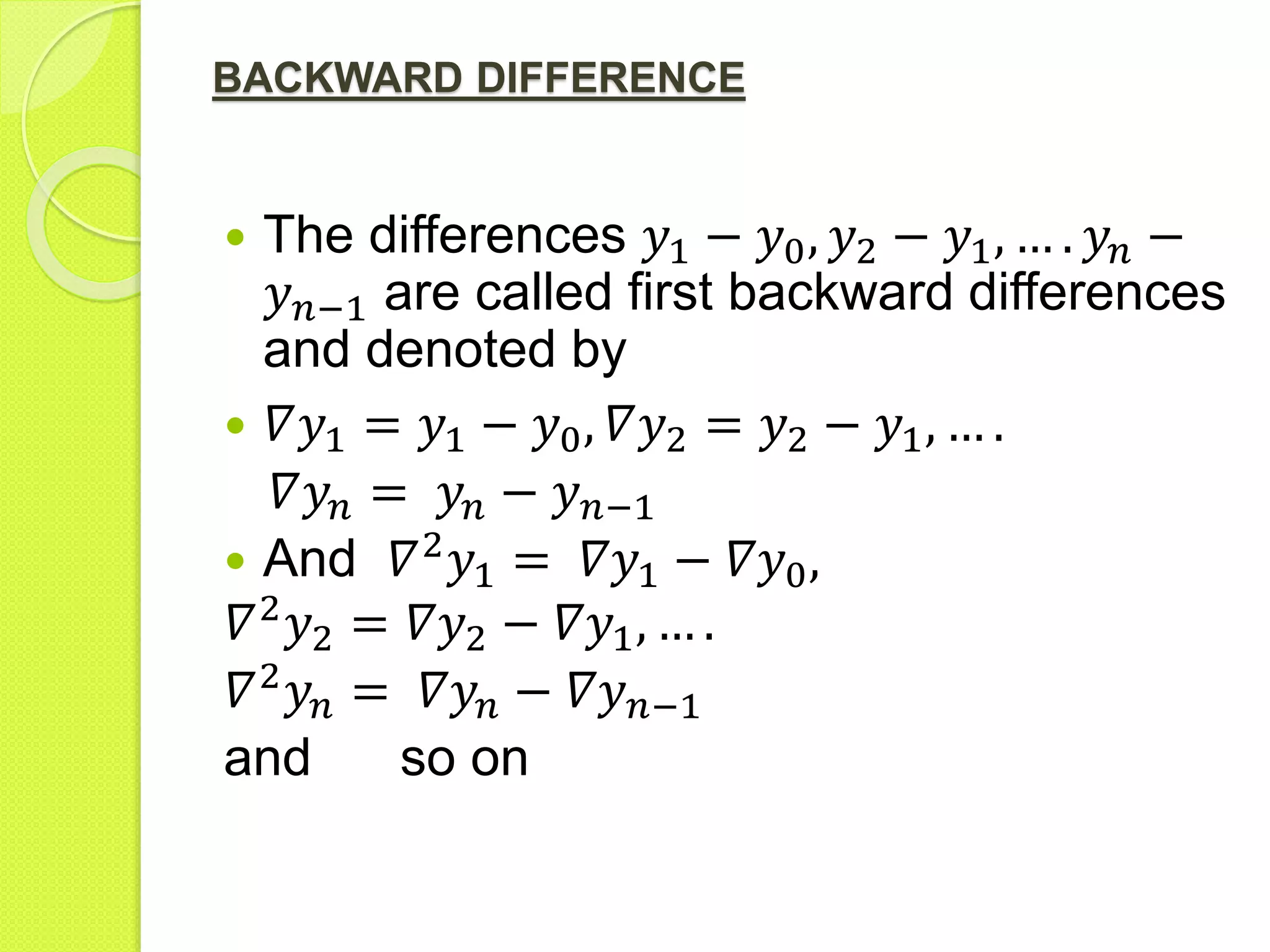
An explanation of first backward differences, noting their notation and calculation from known points.
Formula to estimate values using Newton's backward difference interpolation approach.
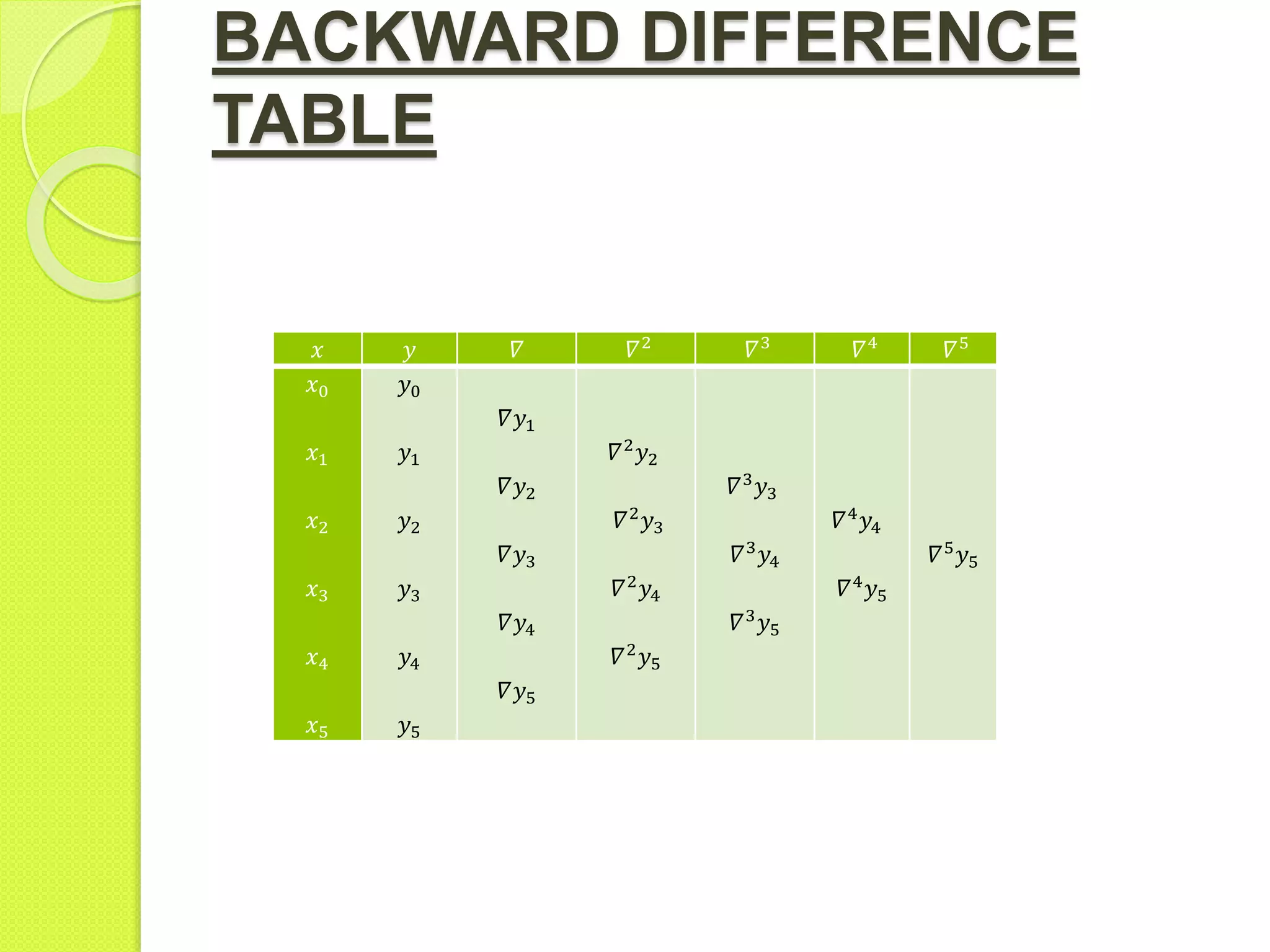
A structured backward difference table for organizing function values and their differences.
Introduction to methods for numerical differentiation, based on interpolation principles.
Stepwise procedure to compute derivatives using Newton’s divided difference formula.
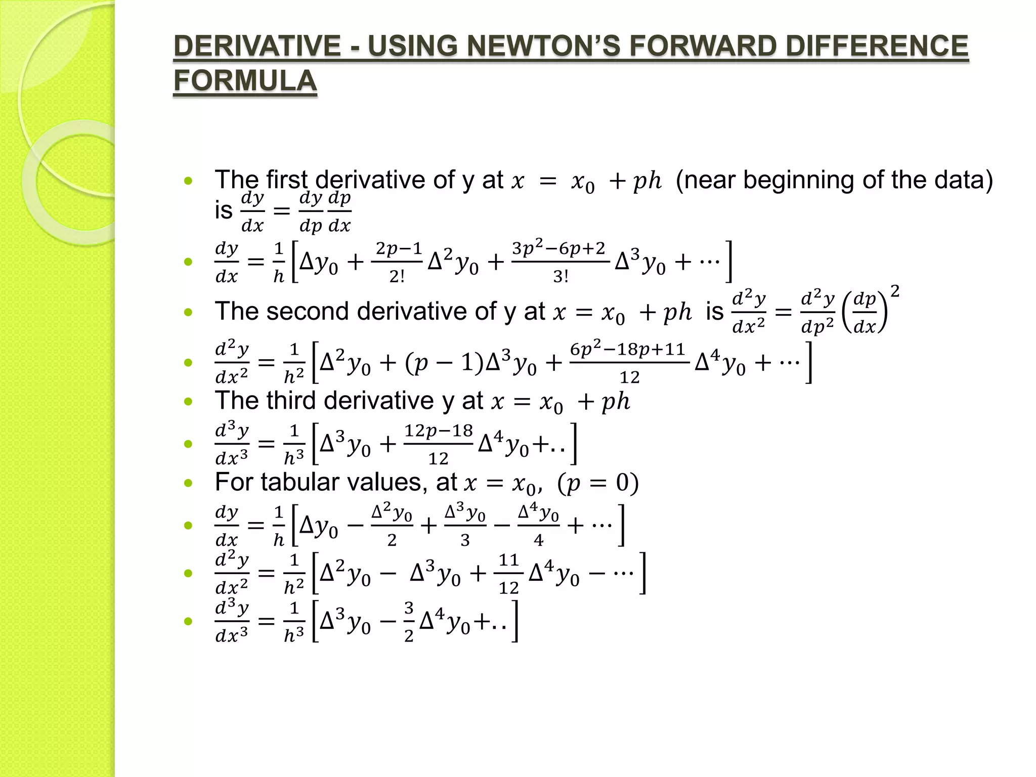
Formulae for calculating first and higher-order derivatives using Newton's forward difference.
Method for calculating derivatives at the chart's end using Newton's backward formula.
Overview of numerical integration methods, specifically trapezoidal and Simpson’s rule.
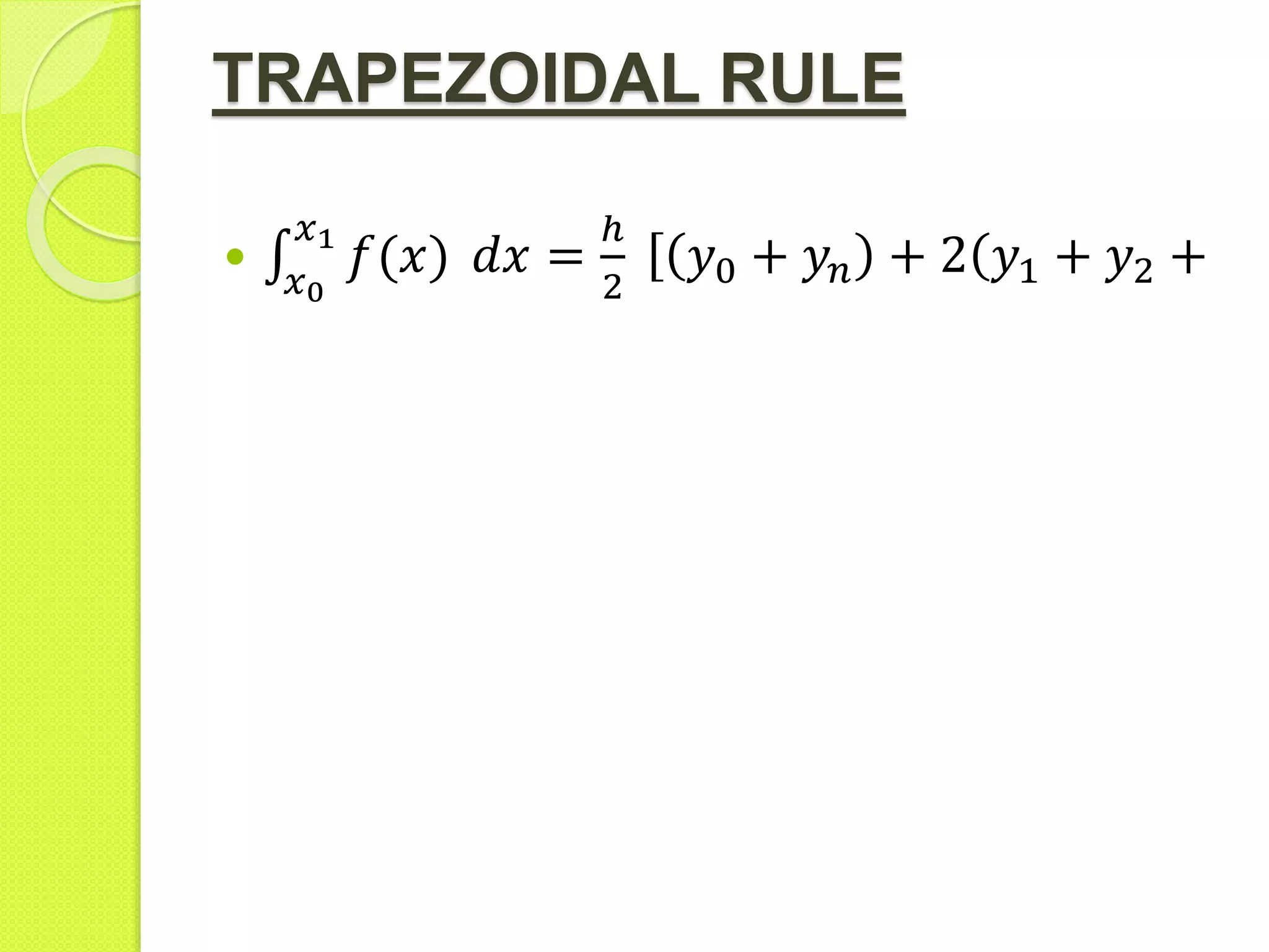
Formula derivation for the integral calculation of a function using the trapezoidal rule.
Integration formula using Simpson's 1/3 rule, detailing even interval requirements for applications.
Introduction to numerical methods for double integrals, addressing trapezoidal and Simpson's rule.
Trapezoidal rule application for double integrals, emphasizing corner and boundary value calculations.
Explanation of Simpson's rule for double integrals, detailing corner and boundary contributions.
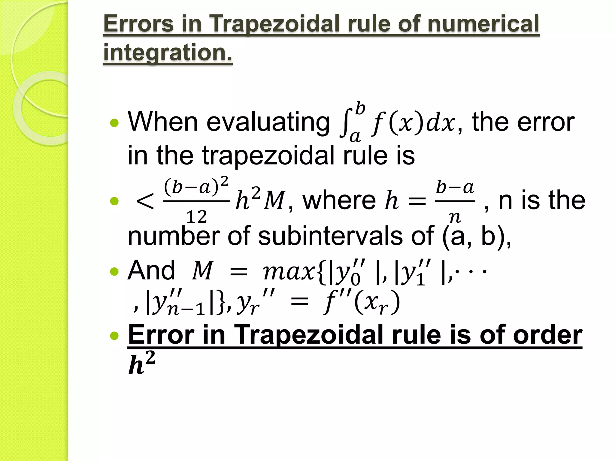
Analysis of error estimates for trapezoidal rule in numerical integration with conditions on intervals.
Error estimation for Simpson's rule, providing conditions for integration accuracy using subintervals.