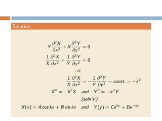
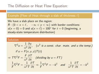
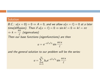
This document discusses various types of partial differential equations (PDEs) relevant in mathematical physics, including Laplace's equation, the heat flow equation, and the wave equation. It provides examples demonstrating how to solve these equations, particularly in context to steady-state temperature distributions and vibrations in a string. The document also explains the Fourier series as a method for approximating functions relevant to these equations.

1. Partial Differential Equations,
Part I
2015.11.19 Enrique Valderrama, Ph.D.

2. Table of contents
1 Introduction
2 Laplace’s Equation
Steady-State temperature in a rectangular plate
Math. Parenthesis: The Fourier Series
3 The Diffusion or Heat Flow Equation
Flow of Heat through a slab of thickness
4 The Wave Equation
The Vibrating String

3. Introduction
Many of the problems of mathematical physics involve the solution
of PDE’s. The same PDE may apply to a variety of physical
problems; then many of the methods will apply to a bigger set of
problems.
Laplace’s Equation: 2
u = 0
Poisson’s Equation: 2
u = f (x, y, z)
The difussion or heat flow equation: 2
u =
1
α2
∂u
∂t
Wave equation: 2
u =
1
v2
∂2u
∂t2
Helmoltz equation: 2
F + k2
F = 0
Schröedinger equation: −
2
2m
2
Ψ + V Ψ = i
∂
∂t
Ψ

4. Laplace’s Equation:
Example (Steady-State temperature in a rectangular plate)
We have a rectangular plate on the region:
R : {0 < x < 10 , 0 < y} with border conditions:
T(x = 0) = T(x = 10) = T(y = ∞) = 0◦ and T(y = 0) = 100◦
Solution
2
T = 0
∂2T
∂x2
+
∂2T
∂y2
= 0
T(x, y) = X(x)Y (y)
Y
∂2X
∂x2
+ X
∂2Y
∂y2
= 0

5. Solution
Y
∂2X
∂x2
+ X
∂2Y
∂y2
= 0
1
X
∂2X
∂x2
+
1
Y
∂2Y
∂y2
= 0
⇒
1
X
∂2X
∂x2
= −
1
Y
∂2Y
∂y2
= const. = −k2
X = −k2
X and Y = +k2
Y
(soln’s:)
X(x) = A cos kx + B sin kx and Y (y) = Ceky
+ De−ky

6. Solution
T(x, y) = X(x)Y (y) = (A cos kx + B sin kx)(Ceky
+ De−ky
)
B.C. : T(x, ∞) = 0 ⇒ C = 0
T(0, y) = 0 ⇒ A = 0 and
T(10, y) = 0 ⇒ sin 10k = 0 ⇒ k = n
π
10
)
⇒
T(x, y) = BD sin n
π
10
x e−n π
10
y
andT(x, 0) = 100 ⇒ BD sin n
π
10
x · 1 = 100

7. Solution
T(x, y) =
∞
n=1
bne−n π
10
y
sin n
π
10
x
For y = 0, we must have T = 100, then :
T(x, 0) =
∞
n=1
bn sin n
π
10
x
which is just the Fourier sine series · · ·

8. Fourier Series:
Similar to Taylor series, which we approx. a function using the
summation of the derivatives of the function and polynomials, a
Fourier series will approx. a function with the summation of cosine
and sine functions:
f (x) = a0 +
∞
k=1
an cos
nπx
+ bn sin
nπx
where the coefficients are given by the Euler formulas
a0 =
1
2 −
f (x) dx,
an =
1
−
f (x) cos
nπx
dx, n = 1, 2, · · ·
bn =
1
−
f (x) sin
nπx
dx, n = 1, 2, · · ·

9. Approximation to a square wave
Considere the square wave, which first wave is:
f = 4 if 0 ≤ x ≤ π
f = 0 if π < x < 2π
and so on
Example
Use FS to approximate the square wave function.
Solution
The Euler coefficients:
a0 =
1
2 −
f (x) dx =
1
2π
0
−π
0 dx +
π
0
4 dx = 2

10. Solution
an =
1
−
f (x) cos
nπx
dx =
1
π
0
−π
0 dx +
π
0
4 cos
nπx
π
dx
=
1
π
π
0
4 cos nx dx =
1
π
4 sin nx
n
π
0
= 0
bn =
1
−
f (x) sin
nπx
dx =
1
π
0
−π
0 dx +
π
0
4 sin
nπx
π
dx
=
1
π
π
0
4 sin nx dx = −
1
π
4 cos nx
n
π
0
=
4
πn
(1 − cos nπ)
⇒
f (x) = 2 +
8
π
sin x +
8
3π
sin 3x +
8
5π
sin 5x + · · ·

11. Let’s come back to Laplace PDE · · ·
Solution
T(x, 0) = 100 =
∞
n=1
bn sin n
π
10
x
We recognize f (x) = 100, = 10 therefore bn are given by:
bn =
1
10
0
−10
0 · sin
nπx
10
dx +
10
0
100 sin
nπx
10
dx
= 10
10
πn
−
10 cos πn
πn
=
200
nπ
, n = 1, 3, 5 · · ·
Finally:
T(x, y) =
∞
n=1
bne−n π
10
y
sin n
π
10
x
=
200
π
e− π
10
y
sin
π
10
x +
1
3
e−3π
10
y
sin
3π
10
x + · · ·

12. The Diffusion or Heat Flow Equation:
Example (Flow of Heat through a slab of thickness )
We have a slab place on the region:
R : {0 < x < , −∞ < y < ∞} with border conditions:
u(x = 0) = 0 and u(x = ) = 100◦ for t = 0 (beginning, a
steady-state temperature distribution)
Solution
2
u =
1
α2
∂u
∂t
, (α2
is a const. char. mate. and u the temp.)
if u = F(x, y, z)T(t)
⇒ T 2
F =
F
α2
∂T
∂t
(dividing by u = FT)
1
F
2
F =
1
α2T
∂T
∂t
⇒
1
F
2
F = −k2
and
1
α2T
∂T
∂t
= −k2

13. Solution
The solution of the DFQ dependent of the time is trivial:
T(t) = e−k2α2t
and in our particular problem, where we have a very long slab, the
diffusion will be only on the x-direction, then the DFQ dependent
on the space coordinates, also become trivial, because we
recognize as the SHO.
∂2F(x)
∂x2
+ k2
F(x) = 0
soln :
F(x) =A cos kx + B sin kx

14. Solution
B.C.: u(x = 0) = 0 ⇒ A = 0, and we allow u(x = ) = 0 at a later
time(diffusion). Then if u(x = ) = 0 ⇒ sin k = 0 ⇒ k = nπ
⇒ k =
nπ
(eigenvalues)
Then our base functions (eigenfunctions) are then
u = e−k2α2t
sin
nπx
and the general solution to our problem will be the series:
u =
∞
n=1
bne−k2α2t
sin
nπx

15. Solution
The problem say at the beginning, a steady-state temperature
distribution is on the slab, which implies u0 satisfy Laplace’s
equation, i.e 2u0 = 0, i.e.
∂u2
0
∂x2 = 0, and the solution for this
equation is u0 = ax + b, then applying border condition we get
u0 =
100
x
Then for t = 0, u(x, t = 0) = u0, i.e.
u(x, t = 0) =
∞
n=1
bn sin
nπx
=
100
x
Which can be solved using F.S., for f (x) = 100
x and the
half-period equal to

16. Solution
The Euler coefficients:
an = 0 (we dont want solutions with cosine functions (B.C.))
bn =
1
−
f (x) sin
nπx
dx =
1 0
−
0 dx +
0
100
x sin
nπx
dx
=
100
2
π
0
x sin
nπx
dx ⇒ (Integration by parts:)
bn =
100(sin πn − πn cos πn)
π2n2
=
100
π
(−1)n−1
n
⇒
u =
100
π
∞
n=1
(−1)n−1
n
e−k2α2t
sin
nπx

17. The Wave Equation:
Example (The Vibrating String)
Let a string be stretched tightly and its ends fastened to supports
at x = 0 and x = . When the string is vibrating, its vertical
displacement y from its equilibrium position along the x-axis
depends on x and t. We assume the displacement y is very small
and that the slope ∂y/∂t is small at any point at any time.
Solution
∂2y
∂x2
=
1
v2
∂2y
∂t2
, (v = T/µ)
if y = X(x)T(t)
⇒
1
X
∂2X
∂x2
=
1
v2
1
T
∂2T
∂t2
= −k2
(soln’s:)
X(x) = A cos kx + B sin kx and T(t) = C cos kvt + D sin kvt

18. Solution
B.C.: y(x = 0) = 0 ⇒ A = 0,
u(x = ) = 0 ⇒ sin k = 0 ⇒ k = nπ ⇒ k = nπ
(eigenvalues)
Then: y1(x, t) = B sin
nπ
x C cos
nπ
vt + D sin
nπ
vt but at
t = 0 every piece of string is not varying with time, the ∂y/∂t = 0
Then D = 0 as well.
Then our base functions (eigenfunctions) are then
y1 = BC sin
nπ
x cos
nπ
vt
and the general solution to our problem will be the series:
y(x, t) =
∞
n=1
bn sin
nπ
x cos
nπ
vt

19. Solution
Then at t = 0, y(x, t) = y0 = f (x), then
y(x, t = 0) =
∞
n=1
bn sin
nπ
x = f (x)
· · ·