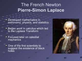
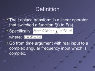
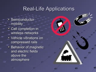
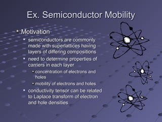
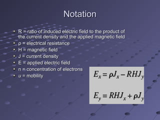
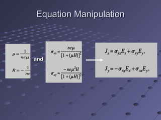
Laplace TransformLaplace Transform
Melissa MeagherMelissa Meagher
Meagan PitluckMeagan Pitluck
Nathan CutlerNathan Cutler
Matt AbernethyMatt Abernethy
Thomas NoelThomas Noel
Scott DrotarScott Drotar
The French Newton
Pierre-Simon Laplace
Developed mathematics in
astronomy, physics, and statistics
Began work in calculus which led
to the Laplace Transform
Focused later on celestial
mechanics
One of the first scientists to
suggest the existence of black
holes
History of the Transform
Euler began looking at integrals as solutions to differential equations
in the mid 1700’s:
Lagrange took this a step further while working on probability
density functions and looked at forms of the following equation:
Finally, in 1785, Laplace began using a transformation to solve
equations of finite differences which eventually lead to the current
transform
Definition
The Laplace transform is a linear operator
that switched a function f(t) to F(s).
Specifically:
where:
Go from time argument with real input to a
complex angular frequency input which is
complex.
RestrictionsRestrictions
There are two governing factors thatThere are two governing factors that
determine whether Laplace transformsdetermine whether Laplace transforms
can be used:can be used:

f(t) must be at least piecewise continuous forf(t) must be at least piecewise continuous for
t ≥ 0t ≥ 0

|f(t)| ≤ Me|f(t)| ≤ Meγγtt
where M andwhere M and γγ are constantsare constants
Since the general form of the LaplaceSince the general form of the Laplace
transform is:transform is:
it makes sense that f(t) must be at leastit makes sense that f(t) must be at least
piecewise continuous for t ≥ 0.piecewise continuous for t ≥ 0.
If f(t) were very nasty, the integral wouldIf f(t) were very nasty, the integral would
not be computable.not be computable.
ContinuityContinuity
BoundednessBoundedness
This criterion also follows directly from theThis criterion also follows directly from the
general definition:general definition:
If f(t) is not bounded by MeIf f(t) is not bounded by Meγγtt
then thethen the
integral will not converge.integral will not converge.
Laplace Transform TheoryLaplace Transform Theory
•General Theory
•Example
•Convergence
Laplace TransformsLaplace Transforms
•Some Laplace Transforms
•Wide variety of function can be transformed
•Inverse Transform
•Often requires partial fractions or other
manipulation to find a form that is easy to
apply the inverse
Laplace Transform for ODEsLaplace Transform for ODEs
•Equation with initial conditions
•Laplace transform is linear
•Apply derivative formula
•Rearrange
•Take the inverse
Laplace Transform in PDEs
Laplace transform in two variables (always taken
with respect to time variable, t):
Inverse laplace of a 2 dimensional PDE:
Can be used for any dimension PDE:
•ODEs reduce to algebraic equations
•PDEs reduce to either an ODE (if original equation dimension 2) or
another PDE (if original equation dimension >2)
The Transform reduces dimension by “1”:
Consider the case where:
ux+ut=t with u(x,0)=0 and u(0,t)=t2
and
Taking the Laplace of the initial equation leaves Ux+ U=1/s2
(note that the
partials with respect to “x” do not disappear) with boundary condition
U(0,s)=2/s3
Solving this as an ODE of variable x, U(x,s)=c(s)e-x
+ 1/s2
Plugging in B.C., 2/s3
=c(s) + 1/s2
so c(s)=2/s3
- 1/s2
U(x,s)=(2/s3
- 1/s2
) e-x
+ 1/s2
Now, we can use the inverse Laplace Transform with respect to s to find
u(x,t)=t2
e-x
- te-x
+ t
Example SolutionsExample Solutions
Diffusion EquationDiffusion Equation
uutt = ku= kuxxxx in (0,l)in (0,l)
Initial Conditions:Initial Conditions:
u(0,t) = u(l,t) = 1, u(x,0) = 1 + sin(πx/l)u(0,t) = u(l,t) = 1, u(x,0) = 1 + sin(πx/l)
UsingUsing af(t) + bg(t)af(t) + bg(t)  aF(s) + bG(s)aF(s) + bG(s)
andand df/dtdf/dt  sF(s) – f(0)sF(s) – f(0)
and noting that the partials with respect to x commute with the transforms withand noting that the partials with respect to x commute with the transforms with
respect to t, the Laplace transform U(x,s) satisfiesrespect to t, the Laplace transform U(x,s) satisfies
sU(x,s) – u(x,0) = kUsU(x,s) – u(x,0) = kUxxxx(x,s)(x,s)
WithWith eeatat
 1/(s-a)1/(s-a) and a=0,and a=0,
the boundary conditions become U(0,s) = U(l,s) = 1/s.the boundary conditions become U(0,s) = U(l,s) = 1/s.
So we have an ODE in the variable x together with some boundary conditions.So we have an ODE in the variable x together with some boundary conditions.
The solution is then:The solution is then:
U(x,s) = 1/s + (1/(s+kπU(x,s) = 1/s + (1/(s+kπ22
/l/l22
))sin(πx/l)))sin(πx/l)
Therefore, when we invert the transform, using the Laplace table:Therefore, when we invert the transform, using the Laplace table:
u(x,t) = 1 + eu(x,t) = 1 + e-kπ-kπ22
t/lt/l22
sin(πx/l)sin(πx/l)
Wave EquationWave Equation
uutttt = c= c22
uuxxxx in 0 < x < ∞in 0 < x < ∞
Initial Conditions:Initial Conditions:
u(0,t) = f(t), u(x,0) = uu(0,t) = f(t), u(x,0) = utt(x,0) = 0(x,0) = 0
For xFor x  ∞, we assume that u(x,t)∞, we assume that u(x,t)  0. Because the initial conditions0. Because the initial conditions
vanish, the Laplace transform satisfiesvanish, the Laplace transform satisfies
ss22
U = cU = c22
UUxxxx
U(0,s) = F(s)U(0,s) = F(s)
Solving this ODE, we getSolving this ODE, we get
U(x,s) = a(s)eU(x,s) = a(s)e-sx/c-sx/c
+ b(s)e+ b(s)esx/csx/c
Where a(s) and b(s) are to be determined.Where a(s) and b(s) are to be determined.
From the assumed property of u, we expect that U(x,s)From the assumed property of u, we expect that U(x,s)  0 as x0 as x  ∞.∞.
Therefore, b(s) = 0. Hence,Therefore, b(s) = 0. Hence, U(x,s) = F(s) eU(x,s) = F(s) e-sx/c-sx/c
. Now we use. Now we use
H(t-b)f(t-b)H(t-b)f(t-b)  ee-bs-bs
F(s)F(s)
To getTo get
u(x,t) = H(t – x/c)f(t – x/c).u(x,t) = H(t – x/c)f(t – x/c).
Real-Life ApplicationsReal-Life Applications
SemiconductorSemiconductor
mobilitymobility
Call completion inCall completion in
wireless networkswireless networks
Vehicle vibrations onVehicle vibrations on
compressed railscompressed rails
Behavior of magneticBehavior of magnetic
and electric fieldsand electric fields
above theabove the
atmosphereatmosphere
Ex. Semiconductor MobilityEx. Semiconductor Mobility
MotivationMotivation

semiconductors are commonlysemiconductors are commonly
made with superlattices havingmade with superlattices having
layers of differing compositionslayers of differing compositions

need to determine properties ofneed to determine properties of
carriers in each layercarriers in each layer
concentration of electrons andconcentration of electrons and
holesholes
mobility of electrons and holesmobility of electrons and holes

conductivity tensor can be relatedconductivity tensor can be related
to Laplace transform of electronto Laplace transform of electron
and hole densitiesand hole densities
NotationNotation
R = ratio of induced electric field to the product ofR = ratio of induced electric field to the product of
the current density and the applied magnetic fieldthe current density and the applied magnetic field
ρ = electrical resistanceρ = electrical resistance
H = magnetic fieldH = magnetic field
J = current densityJ = current density
E = applied electric fieldE = applied electric field
n = concentration of electronsn = concentration of electrons
uu = mobility= mobility
Equation ManipulationEquation Manipulation
andand
Assuming a continuous mobilityAssuming a continuous mobility
distribution and that ,distribution and that ,
, it follows:, it follows:
Applying the Laplace TransformApplying the Laplace Transform
Johnson, William B. Transform method forJohnson, William B. Transform method for
semiconductor mobility, Journal of Appliedsemiconductor mobility, Journal of Applied
Physics 99 (2006).Physics 99 (2006).
Source

Laplace transform

  • 1.
    Laplace TransformLaplace Transform MelissaMeagherMelissa Meagher Meagan PitluckMeagan Pitluck Nathan CutlerNathan Cutler Matt AbernethyMatt Abernethy Thomas NoelThomas Noel Scott DrotarScott Drotar
  • 2.
    The French Newton Pierre-SimonLaplace Developed mathematics in astronomy, physics, and statistics Began work in calculus which led to the Laplace Transform Focused later on celestial mechanics One of the first scientists to suggest the existence of black holes
  • 3.
    History of theTransform Euler began looking at integrals as solutions to differential equations in the mid 1700’s: Lagrange took this a step further while working on probability density functions and looked at forms of the following equation: Finally, in 1785, Laplace began using a transformation to solve equations of finite differences which eventually lead to the current transform
  • 4.
    Definition The Laplace transformis a linear operator that switched a function f(t) to F(s). Specifically: where: Go from time argument with real input to a complex angular frequency input which is complex.
  • 5.
    RestrictionsRestrictions There are twogoverning factors thatThere are two governing factors that determine whether Laplace transformsdetermine whether Laplace transforms can be used:can be used:  f(t) must be at least piecewise continuous forf(t) must be at least piecewise continuous for t ≥ 0t ≥ 0  |f(t)| ≤ Me|f(t)| ≤ Meγγtt where M andwhere M and γγ are constantsare constants
  • 6.
    Since the generalform of the LaplaceSince the general form of the Laplace transform is:transform is: it makes sense that f(t) must be at leastit makes sense that f(t) must be at least piecewise continuous for t ≥ 0.piecewise continuous for t ≥ 0. If f(t) were very nasty, the integral wouldIf f(t) were very nasty, the integral would not be computable.not be computable. ContinuityContinuity
  • 7.
    BoundednessBoundedness This criterion alsofollows directly from theThis criterion also follows directly from the general definition:general definition: If f(t) is not bounded by MeIf f(t) is not bounded by Meγγtt then thethen the integral will not converge.integral will not converge.
  • 8.
    Laplace Transform TheoryLaplaceTransform Theory •General Theory •Example •Convergence
  • 9.
    Laplace TransformsLaplace Transforms •SomeLaplace Transforms •Wide variety of function can be transformed •Inverse Transform •Often requires partial fractions or other manipulation to find a form that is easy to apply the inverse
  • 10.
    Laplace Transform forODEsLaplace Transform for ODEs •Equation with initial conditions •Laplace transform is linear •Apply derivative formula •Rearrange •Take the inverse
  • 11.
    Laplace Transform inPDEs Laplace transform in two variables (always taken with respect to time variable, t): Inverse laplace of a 2 dimensional PDE: Can be used for any dimension PDE: •ODEs reduce to algebraic equations •PDEs reduce to either an ODE (if original equation dimension 2) or another PDE (if original equation dimension >2) The Transform reduces dimension by “1”:
  • 12.
    Consider the casewhere: ux+ut=t with u(x,0)=0 and u(0,t)=t2 and Taking the Laplace of the initial equation leaves Ux+ U=1/s2 (note that the partials with respect to “x” do not disappear) with boundary condition U(0,s)=2/s3 Solving this as an ODE of variable x, U(x,s)=c(s)e-x + 1/s2 Plugging in B.C., 2/s3 =c(s) + 1/s2 so c(s)=2/s3 - 1/s2 U(x,s)=(2/s3 - 1/s2 ) e-x + 1/s2 Now, we can use the inverse Laplace Transform with respect to s to find u(x,t)=t2 e-x - te-x + t
  • 13.
  • 14.
    Diffusion EquationDiffusion Equation uutt= ku= kuxxxx in (0,l)in (0,l) Initial Conditions:Initial Conditions: u(0,t) = u(l,t) = 1, u(x,0) = 1 + sin(πx/l)u(0,t) = u(l,t) = 1, u(x,0) = 1 + sin(πx/l) UsingUsing af(t) + bg(t)af(t) + bg(t)  aF(s) + bG(s)aF(s) + bG(s) andand df/dtdf/dt  sF(s) – f(0)sF(s) – f(0) and noting that the partials with respect to x commute with the transforms withand noting that the partials with respect to x commute with the transforms with respect to t, the Laplace transform U(x,s) satisfiesrespect to t, the Laplace transform U(x,s) satisfies sU(x,s) – u(x,0) = kUsU(x,s) – u(x,0) = kUxxxx(x,s)(x,s) WithWith eeatat  1/(s-a)1/(s-a) and a=0,and a=0, the boundary conditions become U(0,s) = U(l,s) = 1/s.the boundary conditions become U(0,s) = U(l,s) = 1/s. So we have an ODE in the variable x together with some boundary conditions.So we have an ODE in the variable x together with some boundary conditions. The solution is then:The solution is then: U(x,s) = 1/s + (1/(s+kπU(x,s) = 1/s + (1/(s+kπ22 /l/l22 ))sin(πx/l)))sin(πx/l) Therefore, when we invert the transform, using the Laplace table:Therefore, when we invert the transform, using the Laplace table: u(x,t) = 1 + eu(x,t) = 1 + e-kπ-kπ22 t/lt/l22 sin(πx/l)sin(πx/l)
  • 15.
    Wave EquationWave Equation uutttt= c= c22 uuxxxx in 0 < x < ∞in 0 < x < ∞ Initial Conditions:Initial Conditions: u(0,t) = f(t), u(x,0) = uu(0,t) = f(t), u(x,0) = utt(x,0) = 0(x,0) = 0 For xFor x  ∞, we assume that u(x,t)∞, we assume that u(x,t)  0. Because the initial conditions0. Because the initial conditions vanish, the Laplace transform satisfiesvanish, the Laplace transform satisfies ss22 U = cU = c22 UUxxxx U(0,s) = F(s)U(0,s) = F(s) Solving this ODE, we getSolving this ODE, we get U(x,s) = a(s)eU(x,s) = a(s)e-sx/c-sx/c + b(s)e+ b(s)esx/csx/c Where a(s) and b(s) are to be determined.Where a(s) and b(s) are to be determined. From the assumed property of u, we expect that U(x,s)From the assumed property of u, we expect that U(x,s)  0 as x0 as x  ∞.∞. Therefore, b(s) = 0. Hence,Therefore, b(s) = 0. Hence, U(x,s) = F(s) eU(x,s) = F(s) e-sx/c-sx/c . Now we use. Now we use H(t-b)f(t-b)H(t-b)f(t-b)  ee-bs-bs F(s)F(s) To getTo get u(x,t) = H(t – x/c)f(t – x/c).u(x,t) = H(t – x/c)f(t – x/c).
  • 16.
    Real-Life ApplicationsReal-Life Applications SemiconductorSemiconductor mobilitymobility Callcompletion inCall completion in wireless networkswireless networks Vehicle vibrations onVehicle vibrations on compressed railscompressed rails Behavior of magneticBehavior of magnetic and electric fieldsand electric fields above theabove the atmosphereatmosphere
  • 17.
    Ex. Semiconductor MobilityEx.Semiconductor Mobility MotivationMotivation  semiconductors are commonlysemiconductors are commonly made with superlattices havingmade with superlattices having layers of differing compositionslayers of differing compositions  need to determine properties ofneed to determine properties of carriers in each layercarriers in each layer concentration of electrons andconcentration of electrons and holesholes mobility of electrons and holesmobility of electrons and holes  conductivity tensor can be relatedconductivity tensor can be related to Laplace transform of electronto Laplace transform of electron and hole densitiesand hole densities
  • 18.
    NotationNotation R = ratioof induced electric field to the product ofR = ratio of induced electric field to the product of the current density and the applied magnetic fieldthe current density and the applied magnetic field ρ = electrical resistanceρ = electrical resistance H = magnetic fieldH = magnetic field J = current densityJ = current density E = applied electric fieldE = applied electric field n = concentration of electronsn = concentration of electrons uu = mobility= mobility
  • 19.
  • 20.
    Assuming a continuousmobilityAssuming a continuous mobility distribution and that ,distribution and that , , it follows:, it follows:
  • 21.
    Applying the LaplaceTransformApplying the Laplace Transform
  • 22.
    Johnson, William B.Transform method forJohnson, William B. Transform method for semiconductor mobility, Journal of Appliedsemiconductor mobility, Journal of Applied Physics 99 (2006).Physics 99 (2006). Source

Editor's Notes

  • #3 A French mathematician and astronomer from the late 1700’s. His early published work started with calculus and differential equations. He spent many of his later years developing ideas about the movements of planets and stability of the solar system in addition to working on probability theory and Bayesian inference. Some of the math he worked on included: the general theory of determinants, proof that every equation of an even degree must have at least one real quadratic factor, provided a solution to the linear partial differential equation of the second order, and solved many definite integrals. He is one of only 72 people to have his name engraved on the Eiffel tower.
  • #4 Laplace also recognized that Joseph Fourier&amp;apos;s method of Fourier series for solving the diffusion equation could only apply to a limited region of space as the solutions were periodic. In 1809, Laplace applied his transform to find solutions that diffused indefinitely in space