Downloaded 224 times


![
Ex 1: Matrix Size
]2[
00
00
−
2
1
031
− 47
22
πe
11×
22×
41×
23×
Note:
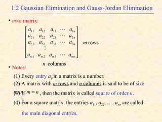
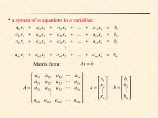
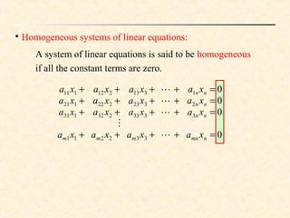
One very common use of matrices is to represent a system
of linear equations.](https://image.slidesharecdn.com/ch1-161103181742/85/System-Of-Linear-Equations-6-320.jpg)
![
Augmented matrix:
][3
2
1
321
3333231
2232221
1131211
bA
b
b
b
b
aaaa
aaaa
aaaa
aaaa
mmnmmm
n
n
n
=
A
aaaa
aaaa
aaaa
aaaa
mnmmm
n
n
n
=
321
3333231
2232221
1131211
Coefficient matrix:](https://image.slidesharecdn.com/ch1-161103181742/85/System-Of-Linear-Equations-8-320.jpg)


The document provides an introduction to systems of linear equations, detailing their characteristics, including potential solutions and equivalent systems. It covers Gaussian elimination and Gauss-Jordan elimination techniques for solving these systems, emphasizing matrix representation and elementary row operations. Additionally, it discusses homogeneous systems, their solutions, and the concepts of trivial and nontrivial solutions.