This document provides an introduction and overview of the Laplace transform method for solving differential equations. It defines the Laplace transform and lists some of its key properties. It then provides examples of using the Laplace transform method to solve problems involving the deflection of beams under different loading conditions. Specifically, it shows how to use the Laplace transform to find the deflection of a beam with uniform distributed load that is simply supported at both ends. The resulting equation provides the deflection as a function of position along the beam.

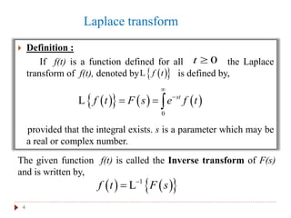
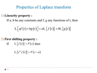
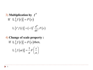
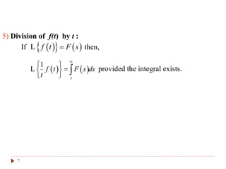
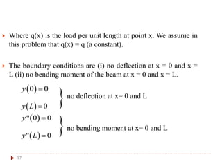
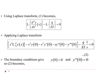
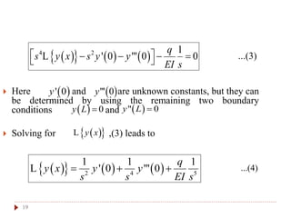
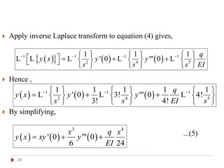
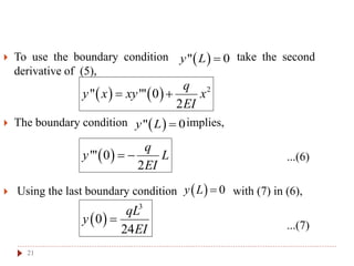
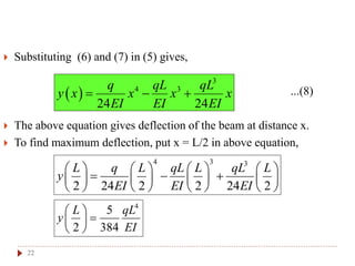
1. 1
Laplace Transform
And
Its Application
Prepare by:
Mayur prajapati

2. 2
Outline
 Introduction
 Laplace transform
 Properties of Laplace transform
 Transform of derivatives
 Deflection of Beam
 Reference

3. 3
Introduction
 The Laplace transform method is powerful method for solving
linear ODEs and corresponding initial value problems, as well
as systems of ODEs arising in engineering.
 This method has two main advantages over usual methods of
ODEs :
1) Problems are solved more directly, IVP without first
determining general solution, and non-homogeneous ODEs
without first solving the corresponding homogeneous ODE.
2) The use of Unit step function (Heaviside function) and
Dirac’s delta make the method particularly powerful for
problems with inputs (driving force) that have discontinuities
or represent short impulse or complicated periodic function.

4. 4
Laplace transform
 Definition :
If f(t) is a function defined for all the Laplace
transform of f(t), denoted by is defined by,
provided that the integral exists. s is a parameter which may be
a real or complex number.
0t 
  f tL
      
0
st
f t F s e f t


  L
    1
f t F s
 L
The given function f(t) is called the Inverse transform of F(s)
and is written by,

5. 5
Properties of Laplace transform
1) Linearity property :
If a, b be any constants and f, g any functions of t, then
2) First shifting property :
If then
         af t bg t a f t b g t    L L L
    f t F sL
    at
e f t F s a L

6. 6
3) Multiplication by
If
4) Change of scale property :
If then,
n
t
      1
n
nn
n
d
t f t F s
ds
 L
    f t F sL
    f t F sL
   1 s
f at F
a a
 
  
 
L

7. 7
5) Division of f(t) by t :
If then,
provided the integral exists.
    f t F sL
   
1
s
f t F s ds
t

 
 
 
L

8. Transform of derivatives
8
 Laplace transform of the derivative of any order :
Let f, f’, ..., be continuous for all and be
piecewise continuous on every finite interval on the semi-axis
then transform of given by,
n
f
 1n
f 
0t 
n
f
0t 
n
f
         1 2 1
0 ' 0 ... 0n n n n n
f s f s f s f f  
    L L

9. Deflection of Beam
 Consider a beam of length L and rectangular cross section and
homogeneous elastic material (e.g., steel) shown in fig.
 If we apply a load to beam in vertical plane through the axis of
symmetry (the x-axis ) beam is bent.
 It axis is curved into the so called elastic curve or deflection
curve.
 Consider a cross-section of the beam cutting the elastic curve
in P and the neutral surface in the line AA’ .
9

10. 10

11. 11
 The bending moment M about AA’ is given by the Bernoulli-
Euler law,
...(1)
where, E = modulus of elasticity of the beam
I = moment of inertia of the cross-section AA’
R = radius of curvature of the elastic curve at P(x , y)
If the deformation of the beam is small, the slop of the elastic
curve is also small so that we may neglect in the
formula,
EI
M
R

3
2 2
2
2
1
dy
dx
R
d y
dx
  
  
   
2
( / )dy dx

12.  For small deflection,
 Hence,(1) bending moment
 Shear force
 Intensity of loading
 The sum of moments about any section due to external forces
on the left of the section, if anti-clock is taken as positive and if
clockwise is taken as negative.
2
2
d y
M EI
dx

3
3
dM d y
EI
dx dx
 
  
 
 
2 4
2 4
d M d y
EI q x
dx dx
 
   
 
12
2 2
1/ ( / )R d y dx

13. 13
 The most important supports corresponding boundary
conditions are :
1) Simply supported :
 There being no deflection and bending moment. We have,
,
,
 0 0y   " 0 0y 
 " 0y L   0y L 

14. 14
2) Clamped at x=0, free at x=L :
 At x=0, the deflection and slop of the beam being both zero. At
x=L, there are no bending moment and shear force. We have,
,
   0 ' 0 0y y     " "' 0y L y L 

15. 15
3) Clamped at both ends :
The deflection and the slop of the beam being both zero. we have
,
,
 0 0y 
  0y L 
 ' 0 0y 
 ' 0y L 

16. Deflection of Beam Carrying Uniform Distributed Load
16
 A uniformly loaded beam of length L is supported at both ends.
The deflection y(x) is a function of horizontal position x & is
given by the differential equation,
...(1)
4
4
1
( )
d y
q x
dx EI


17. 17
 Where q(x) is the load per unit length at point x. We assume in
this problem that q(x) = q (a constant).
 The boundary conditions are (i) no deflection at x = 0 and x =
L (ii) no bending moment of the beam at x = 0 and x = L.
no deflection at x= 0 and L
no bending moment at x= 0 and L
 " 0 0y 
  0y L 
 " 0y L 
 0 0y 



18. 18
 Using Laplace transform, (1) becomes,
 Applying Laplace transform
...(2)
 The boundary conditions give and
so (2) becomes,
 
4
4
0
d y q
x
dx EI
   
    
  
L L
          4 3 2 1
0 ' 0 " 0 "' 0 0
q
s y x s y s y sy y
EI s
       L
 0 0y   " 0 0y 

19. 19
...(3)
 Here and are unknown constants, but they can
be determined by using the remaining two boundary
conditions and
 Solving for ,(3) leads to
...(4)
      4 2 1
' 0 "' 0 0
q
s y x s y y
EI s
     L
 ' 0y  "' 0y
  0y L   " 0y L 
      2 4 5
1 1 1
' 0 "' 0
q
y x y y
s s EI s
  L
  y xL

20. 20
 Apply inverse Laplace transform to equation (4) gives,
 Hence ,
 By simplifying,
...(5)
      1 1 1 1
2 4 5
1 1 1
' 0 "' 0
q
y x y y
s s s EI
                        
L L L L L
     1 1 1
2 4 5
1 1 1 1 1
' 0 3! "' 0 4!
3! 4!
q
y y
s s
y x
EI s
       
      
     
L L L
     
3 4
' 0 "' 0
6 24
x q x
y x xy y
EI
  

21. 21
 To use the boundary condition take the second
derivative of (5),
 The boundary condition implies,
...(6)
 Using the last boundary condition with (7) in (6),
...(7)
 " 0y L 
    2
" "' 0
2
q
y x xy x
EI
 
 " 0y L 
 "' 0
2
q
y L
EI
 
  0y L 
 
3
0
24
qL
y
EI


22. 22
 Substituting (6) and (7) in (5) gives,
...(8)
 The above equation gives deflection of the beam at distance x.
 To find maximum deflection, put x = L/2 in above equation,
 
3
4 3
24 24
q qL qL
y x x x x
EI EI EI
  
4 3 3
2 24 2 2 24 2
L q L qL L qL L
y
EI EI EI
       
         
       
4
5
2 384
L qL
y
EI
 
 
 

23. Reference
23
 Advanced Engineering Mathematics 9th e, Erwin Kreyzig, 2014
 Higher Engineering Mathematics, B. S. Grewal, 1998

24. 24
THANK YOU