Trnasformada de LAplace

1. Laplace Transforms
1. Introduction ……………………………………. 1
2. Definition ………………………………………. 2
3. Properties of the Laplace Transform …………… 4
4. Inverse Laplace Transforms …………………… 6
5. Using Laplace Transforms to Solve ODEs ……. 9
6. The Step Function ……………………………... 11
7. The Dirac Delta Function ……………………… 20
8. Convolution ……………………………………. 25
9. A Note on Control Theory …………………….. 26
Tutorial Exercises ……………………………… 27
Answers to Tutorial Exercises …………………. 33
SCHOOL OF ENGINEERING & BUILT
ENVIRONMENT
Mathematics

2. 1
Laplace Transforms
1) Introduction
The idea of transforming a “difficult” problem into an “easier” problem is one that is used
widely in mathematics. Diagrammatically we have
Problem Transformed
Problem
Solution Transformed
Solution
Transform
Solve
Inverse
Transform
Difficult
There are many types of transforms available to mathematicians, engineers and scientists. We
are going to examine one such transformation, the Laplace transform, which can be used to
solve certain types of differential equations and also has applications in control theory.
2) Definition
The Laplace transform operates on functions of t . Given a function )(tf we define its
Laplace transform as

∞
−
=
0
)(])([ dtetftfL ts
where s is termed the Laplace variable. We sometimes denote the Laplace transform by
)( sF or f .
We start off with a function of t and end up with a function of s ; s is, in fact, a complex
variable, but this need not concern us too much.
Because the function of t is often some form of time signal, we often talk about moving from
the time domain to the Laplace domain when we perform a Laplace transformation.
Note: Laplace transforms are only concerned with functions where 0≥t .

3. 2
Examples
(1) 1)( =tf :
∞=
=
−
∞
−






−=
= 
t
t
ts
ts
e
s
dteL
0
0
1
.1]1[
Strictly speaking, we can’t set t equal to ∞, but we can “take the limit” as t heads
towards infinity. Providing 0>s , thereby ensuring that we have a negative
exponential, the limit of the inside of the square brackets as t tends to infinity will be
zero. Also, since 10
=e , this leaves us with
ss
L
11
0]1[ =





−−= .
So 1)( =tf →
s
L
1
]1[ =
(2) ttf =)( :

∞
−
=
0
.][ dtettL ts
This integral requires integration by parts to complete the process, but with the same
assumptions regarding s as before, it can readily be shown that
2
1
][
s
tL = .
So ttf =)( → 2
1
][
s
tL =
Very quickly the integrations required to complete the Laplace transformation become
difficult and messy. For this reason, we generally work from a table of pre-determined
Laplace transforms (see Appendix).

4. 3
Examples Using Table of Laplace Transforms
(3) (a) Determine ][ 3
tL .
3
t is not in the table explicitly, but n
t is:
1
!
][ +
= n
n
s
n
tL
For 3
t we require 3=n :
444
3 6123!3
][
sss
tL =
××
==
(b) Determine ][ 2t
eL −
.
From table:
α
α
+
=−
s
eL t 1
][ .
Set 2=α :
2
1
][ 2
+
=−
s
eL t
(c) Determine ])4(sin[ tL .
From table:
22
])(sin[
ω
ω
ω
+
=
s
tL .
Set 4=ω :
16
4
4
4
])4(sin[ 222
+
=
+
=
ss
tL

5. 4
3) Properties of the Laplace Transform
The Laplace transform has several special properties that make it a useful mathematical tool.
We consider some of these now.
a) Linearity
Suppose we have two functions along with their respective Laplace transforms:
)(])([ sFtfL = )(])([ sGtgL = .
The property of linearity means that
)()(])()([ sGbsFatgbtfaL +=+
providing a and b are constants. This makes the transformation of a string of functions
straightforward.
Example
(4) 222222
32
32])(sin3)(cos2[
ω
ω
ω
ω
ω
ωω
+
+
=
+
+
+
=+
s
s
ss
s
ttL
Warning: The Laplace transform of a product is NOT EQUAL TO the product of
the individual Laplace transforms. We have to invoke other properties of
the Laplace transform to deal with such.
b) The First Shifting Theorem
Suppose a function )(tf has the Laplace transform )( sF . It is easily demonstrated that
)(])([ αα
+=−
sFtfeL t
.
Example
(5) From tables and Example (3)(a) we have
4
3 6
][
s
tL = . [1]
By the first shifting property
4
32
)2(
6
][
+
=−
s
teL t
. [2]
To obtain [2] from [1] we merely replace s by )2( +s .

6. 5
c) Transformation of Derivatives
As before, denote the Laplace transform (LT) of )(tf by )( sF . Now consider the LT of
the derivative of )(tf , denoted by )(tf :
dtetftfL ts−
∞
= )(])([
0
 .
Integrate by parts (integrating )(tf and differentiating ts
e −
):
[ ] 
∞
−∞−
−−=
00 )()()( dtestfetf tsts

∞
−
+−=
0
)()0(0 dtetfsf ts
)()0( sFsf +−= .
So
)0()(])([ fsFstfL −= .
We have expressed the Laplace transform of a derivative in terms of the Laplace transform of
the undifferentiated function. In effect, the Laplace transform has converted the operation of
differentiation into the simpler operation of multiplication by s .
In a similar fashion, using repeated integration by parts, we can show that
)0()0()(])([ 2
ffssFstfL  −−= .
This is one of the most important properties of the Laplace transform. The Laplace transform
“gets rid of” derivatives; just the thing for solving differential equations!
When we come to solve differential equations using Laplace transforms we shall use the
following alternative notation:
xxL =][
)0(][ xxsxL −=
)0()0(][ 2
xxsxsxL  −−= .
However, before we can solve differential equations, we need to look at the reverse process of
finding functions of t from given Laplace transforms.

7. 6
4) Inverse Laplace Transforms
So far, we have looked at how to determine the LT of a function of t , ending up with a
function of s . The table of Laplace transforms collects together the results we have
considered, and more. When we apply Laplace transforms to solve problems we will have to
invoke the inverse transformation. That is, given a Laplace transform )( sF we will want to
determine the corresponding )(tf . In general we have

∞+
∞−
−
=
j
j
ts
dsesF
j
sFL
γ
γπ
)(
2
1
])([1
,
where the evaluation of the integral requires a knowledge of complex analysis, which is too
difficult to consider here. Instead, we shall rely on the table of Laplace transforms used in
reverse to provide inverse Laplace transforms. This will mean manipulating a given Laplace
transform until it looks like one or more entries in the right of the table. The inverse is then
determined from the left of the table. The following examples illustrate the main algebraic
techniques required. These include completing the square, factorisation and the formation of
partial fractions. See separate documents for the details of completing the square and partial
fractions.
Examples
(6) Invert the Laplace transform 6
3
s
.
The closest entry in the table is 1
!
+n
s
n
which is inverted as:
n
n
t
s
n
→+ 1
!
.
Setting 5=n :
5
6
!5
t
s
→ . [Note: 12012345!5 =××××= ], so 5
6
120
t
s
→ .
In the given Laplace transform there is a 3 in the numerator but we would like there to
be a 120 to match the table entry. We can re-write the transform providing we do not
alter its “net value”:






=== 6666
120
40
1120
120
31
3
3
ssss
.
The term in the square brackets is now exactly the table entry so we can invert that and
simply multiply by the fraction in front:
5
6
40
13
t
s
→ .

8. 7
(7) Invert
52
1
2
++ ss
.
This requires the technique of “completing the square” and a little bit of fine tuning to
re-write it in a form that can be inverted from tables. Note that the closest entry in the
table gives:
)(sin
)( 22
te
s
t
ω
ωα
ω α−
→
++
.
Now complete the square in the denominator:
4)1(51)1(52 222
++=+−+=++ ssss .
The given transform becomes:
2222
2)1(
1
4)1(
1
52
1
++
=
++
=
++ ssss
.
This is now very close to the table entry with 1=α and 2=ω . We would like there
to be a 2 on top so “fine tuning” gives






++
=
++ 2222
2)1(
2
2
1
2)1(
1
ss
,
where the term in the square brackets is exactly the table entry with 1=α and 2=ω .
Inverting this and multiplying by the fraction gives
)2(sin
2)1(
2
2
1
2
1
22
te
s
t−
→





++
.
(8)(a) Invert
32
5
2
−−
+
ss
s
.
Factorising the denominator and splitting the result into its partial fractions deals with
this one. Note that the details of the partial fraction expansion have been omitted.
1
1
3
2
)1()3(
5
32
5
2
+
−
−
=
+−
+
=
−−
+
ssss
s
ss
s
Use t
e
s
α
α
−
→
+ )(
1
twice with 3−=α and 1+=α to give
tt
ee
ss
−
−→
+
−
−
3
2
1
1
3
2

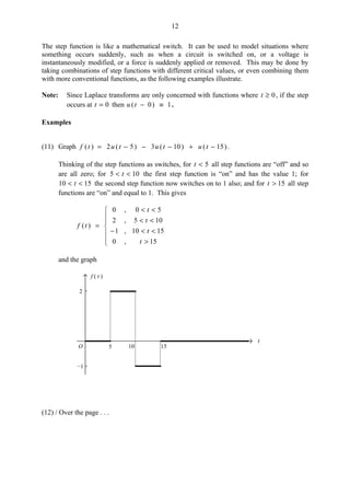
9. 8
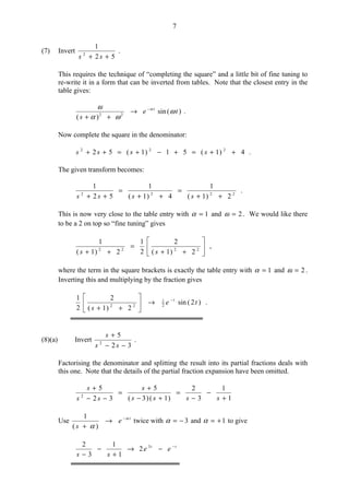
(8)(b) Invert
32
5
2
−−
+
ss
s
by completing the square.
If we failed to notice that the denominator factorised, them completing the square is still
an option:
22
2
22
2)1(
5
4)1(
5
31)1(
5
32
5
−−
+
=
−−
+
=
−−−
+
=
−−
+
s
s
s
s
s
s
ss
s
The minus sign in the denominator is very significant since it no longer conforms to
22
)( ωα ++s .
Instead we need the following results:
22
)(
])(sinh[
βα
β
βα
−+
=−
s
teL t
22
)(
])(cosh[
βα
α
βα
−+
+
=−
s
s
teL t
where sinh (pronounced “shine”) and cosh (pronounced “cosh”) are the so-called
hyperbolic functions. Fine tuning the Laplace transform a little bit more gives
.
2)1(
2
3
2)1(
)1(
2)1(
6)1(
2)1(
5
22222222 





−−
+





−−
−
=
−−
+−
=
−−
+
ss
s
s
s
s
s
Inverting now gives
.])2(sinh3)2(cosh[
)2(sinh3)2(cosh
2)1(
2
3
2)1(
)1(
2222
tte
tete
ss
s
t
tt
+=
+→





−−
+





−−
−
+
++
By applying the following mathematical identities:
][)(cosh 2
1 tt
eet ββ
β −+
+= and ][)(sinh 2
1 tt
eet ββ
β −+
−=
we can easily show that the two versions of the answer are equivalent.

10. 9
5) Using Laplace Transforms to Solve ODEs
We have seen how the Laplace transform of the derivative of a function can be expressed in
terms of the Laplace transform of the undifferentiated function. We can use this property to
derive solutions to certain types of differential equations. The process is broken down into
the following steps:
• Transform both sides of the ODE;
• Substitute initial values;
• Solve for x ;
• Manipulate into a form that can be inverted from tables;
• Invert to give the solution of the ODE.
The method is best illustrated by example and we shall need the results from earlier:
xxL =][
)0(][ xxsxL −=
)0()0(][ 2
xxsxsxL  −−= .
Example
(9) Consider the ODE
t
exxx 3
852 −
=++ 
Subject to the initial conditions
0)0()0( == xx  .
Transform both sides of the equation:
3
8
5])0([2])0()0([ 2
+
=+−+−−
s
xxxsxxsxs  .
Substitute initial values:
3
8
5]0[2]00[ 2
+
=+−+−−
s
xxssxs
3
8
)52( 2
+
=++
s
xss .

11. 10
Solve for x :
)52()3(
8
2
+++
=
xss
x .
Manipulate into a form that can be inverted from tables. In this case we form partial
fractions, complete the square on the quadratic denominator and finish up with a little
“fine tuning” of the last term:






++
+





++
−





+
= 2222
2)1(
2
2
1
2)1(3
1
ss
s
s
x .
Finally invert term-by-term and tidy-up:
.])2(sin)2(cos[
)2(sin])2(sin)2(cos[)(
3
2
1
2
13
ttee
tetteetx
tt
ttt
−−=
+−−=
−−
−−−
Further Example
(10) Solve 125 =+ xx subject to 10)0( =x and 0)0( =x .
Transform:
s
xxxsxs
1
25])0()0([ 2
=+−− 
Substitute initial conditions:
s
xsxs
1
25]010[ 2
=+−−
Solve for x :
s
s
xxs 10
1
252
+=+
s
s
xs 10
1
)25( 2
+=+
)25(
10
)25(
1
22
+
+
+
=
s
s
ss
x

12. 11
Manipulate and invert:






+
+





+
=
)25(
10
)25(
25
25
1
22
s
s
ss
x
)5(cos10])5(cos1[)( 25
1
tttx +−=
Using Laplace transforms to solve ODEs of the form
)(tfxcxbxa =++ 
allows us to tackle problems where a solution by the method of undetermined coefficients
(say) is rendered difficult or impossible because of the specific type of function on the right-
hand-side. We shall now look at two such functions for which this is the case.
6) The Step Function
The step function is defined as



>
<
=−
Tt
Tt
Ttu
,1
,0
)( .
Its graph is shown below in Figure 1:
)( Ttu −
O
t
1
T
Figure 1
T is called the critical value of the step function; it is where the function changes value. The
value of the step function at Tt = is not defined above. Some authors define the value as 1,
others define it as 0 or 0.5. We shall not worry about it!
Note: In the notation for the step function, the u is NOT multiplying the bracket. The u is
the short-hand name for the function (full name: unit step function) and the bracket contains
information regarding the function variable (usually t ) and the location of the step.

13. 12
The step function is like a mathematical switch. It can be used to model situations where
something occurs suddenly, such as when a circuit is switched on, or a voltage is
instantaneously modified, or a force is suddenly applied or removed. This may be done by
taking combinations of step functions with different critical values, or even combining them
with more conventional functions, as the following examples illustrate.
Note: Since Laplace transforms are only concerned with functions where 0≥t , if the step
occurs at 0=t then 1)0( ≡−tu .
Examples
(11) Graph )15()10(3)5(2)( −+−−−= tutututf .
Thinking of the step functions as switches, for 5<t all step functions are “off” and so
are all zero; for 105 << t the first step function is “on” and has the value 1; for
1510 << t the second step function now switches on to 1 also; and for 15>t all step
functions are “on” and equal to 1. This gives







>
<<−
<<
<<
=
15,0
1510,1
105,2
50,0
)(
t
t
t
t
tf
and the graph
f ( t )
t
O 5 10 15
2
−1
(12) / Over the page . . .

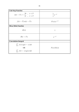
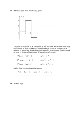
14. 13
(12) Graph ])4()2([)4()2()( −−−−−= tututttf .
We do this in two parts. Without the step functions, we would have
86)4()2()( 2
−+−=−−= tttttf .
This graph is a parabola that crosses the horizontal axis at 2=t and 4=t and has a
maximum turning point at )1,3( .
The step functions take the following values:





>=−
<<=−
<=−
=−−−
4,011
42,101
2,000
)4()2(
t
t
t
tutu .
When the two parts are multiplied together we get





>
<<
<
=
4,0
42,parabola
2,0
)(
t
t
t
tf
and the graph
f ( t )
t
O 2 4
1
We can think of a difference of two step functions
)()( btuatu −−−
like a mathematical window whose frame obscures the graph of any multiplying function to
the sides, i.e. at < and bt > .

15. 14
(13) Determine )(tf from the following graph:
f ( t )
t
O 1 2 3
4
−2
2
The jumps in the graph can be represented by step functions. The location of the jump
is determined by the critical value of the step function, the size of the jump can be
achieved by multiplying the step function be a suitably sized constant, the direction of
the jump by the sign of the constant. Working from left to right:
1st
jump: )1(4 −tu up by 4 at 1=T
2nd
jump: )2(6 −− tu down by 6 at 2=T
3rd
jump: )3(4 −tu up by 4 at 3=T .
Adding these together gives us the function:
)3(4)2(6)1(4)( −+−−−= tutututf .
(14) / Over the page . . .

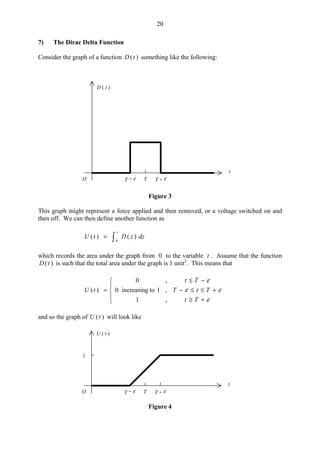
16. 15
(14) Determine )(tf from the following graph:
f ( t )
t
O 1 2
3
Using basic coordinate geometry, the equation of the oblique straight line is given by
33 −= ty .
We are only seeing the straight line between 1=t and 2=t ; this gives a
“mathematical window” of
])2()1([ −−− tutu .
Multiplying the two parts together gives us our function:
])2()1([)33()( −−−−= tututtf .
For more general piece-wise functions we can break them down into fragments, each with
their own window, and add the parts together.
Example
(15)





>
<<−
<<
=
2,0
21,2
10,
)(
t
tt
tt
tf
])2()1([)2(])1()0([)( −−−−+−−−= tututtututtf
As far as Laplace transforms are concerned 1)0( ≡−tu so this can be re-written as
)2()2()1()1(2)( −−+−−−= tuttutttf .

17. 16
There are two results that we will need in order to solve ODEs containing step functions.
Result 1
Ts
e
s
TtuL −
=−
1
])([
Proof
.)0(
1
1
0
10
)(])([
0
0
>=






−+=
+=
−=−
−
∞
−
∞
−−
∞
−


se
s
e
s
dtedte
dteTtuTtuL
Ts
T
ts
T
ts
T
ts
ts
Result 2 – The Second Shifting Theorem
Given a function )(tf with Laplace transform )( sF , it can be shown that
Ts
esFTtuTtfL −
=−− )(])()([ .
The proof of this is omitted. The implication of this result is demonstrated graphically below
in Figure 2:
O O
t t
T
f Shifted and truncated f
)()( tfsF → )()()( TtuTtfesF Ts
−−→−
Figure 2

18. 17
We shall use modified versions of the following diagram to help us apply the 2nd
Shifting
Theorem:
Ts
esFTtuTtf
sFtf
−
↔−−
↔
)()()(
)()(

Examples
(16) Invert the Laplace transform s
e
ss
4
)2(
1 −
+
.
For this we are starting at the bottom-right of the diagram and moving round anti-
clockwise:
Ts
esFTtuTtf
sFtf
−
−−
↑↓
←
)()()(
)()(
Step 1: Ignore exponential to give 





+
=
+
=
)2(
2
2
1
)2(
1
)(
ssss
sF .
Step 2: Invert )( sF to give ]1[)( 2
2
1 t
etf −
−= .
Step 3: Shift and truncate with 4=T , i.e. replace t by )4( −t and multiply by
)4( −tu , to give the completed inversion
)4(]1[)()( )4(2
2
1
−−=−− −−
tueTtuTtf t
.

19. 18
(17) Solve the differential equation )3(4 −=+ tuxx subject to 0)0()0( == xx  .
Transform: s
e
s
xxxsxs 32 1
4])0()0([ −
=+−− 
Substitute initial conditions and solve for x :
s
e
s
xs 32 1
)4( −
=+
s
e
ss
x 3
2
)4(
1 −
+
=
Invert with the help of the 2nd
Shifting Theorem:
Again, we are starting at the bottom-right of the diagram and moving round anti-
clockwise:
Ts
esFTtuTtf
sFtf
−
−−
↑↓
←
)()()(
)()(
Step 1: Ignore exponential to give 





+
=
+
=
)2(
2
4
1
)4(
1
)( 22
2
2
ssss
sF .
Step 2: Invert )(sF to give ])2(cos1[)( 4
1
ttf −= .
Step 3: Shift and truncate with 3=T , i.e. replace t by )3( −t and multiply by
)3( −tu , to give )()( TtuTtf −− and the completed solution
)3(]))3(2(cos1[)( 4
1
−−−= tuttx .
These two examples illustrate the use of the 2nd
Shifting Theorem to invert Laplace
transforms that contain an exponential factor. The next example shows the theorem working
in the other direction.

20. 19
(18) Determine ])10([ 2
−tutL .
This time we go round the diagram the other way:
Ts
esFTtuTtf
sFtf
−
−−
↓↑
→
)()()(
)()(
We have, however, a slight problem in that the given function of t does not quite
conform to the structure bottom-left. We need to re-write the multiplying function 2
t
so that the variable t always has a “minus T ”. For this example 10=T so we
introduce this as follows:
100)10(20)10(]10)10([ 222
+−+−=+−= tttt .
The original function becomes )10(]100)10(20)10([ 2
−+−+− tutt which
now does conform. Next we use the theorem to transform:
Step 1: Cover up the step function and the “minus 10s” to leave
10020)( 2
++= tttf .
Step 2: Transform to give
sss
sF
100202
)( 23
++= .
Step 3: Everything we covered up in Step 1 is now accounted for by multiplying
)(sF by s
e 10−
and so completes the transformation,
s
e
sss
tutL 10
23
2 100202
])10([ −






++=− .
Now we shall look at another new type of function, one that is closely related to the step
function.

21. 20
7) The Dirac Delta Function
Consider the graph of a function )(tD something like the following:
TT − ε T + ε
t
D ( t )
O
Figure 3
This graph might represent a force applied and then removed, or a voltage switched on and
then off. We can then define another function as
=
t
dzzDtU
0
)()(
which records the area under the graph from 0 to the variable t . Assume that the function
)(tD is such that the total area under the graph is 1 unit2
. This means that





+≥
+≤≤−
−≤
=
ε
εε
ε
Tt
TtT
Tt
tU
,1
,1toincreasing0
,0
)(
and so the graph of )(tU will look like
TT − ε T + ε
t
U ( t )
O
1
Figure 4

22. 21
Now suppose that the interval over which )(tD is non-zero is reduced but the height of the
graph is increased in such a way that the total area under the graph is still 1 unit2
:
T
t
D ( t )
O
Figure 5
We get what might be termed a "blip". The corresponding graph of )(tU looks like
T
t
U ( t )
O
1
Figure 6
Notice that )(tU is beginning to look like the step function. If we let the interval about T
shrink further towards zero and the height increase towards infinity (again, in such a way that
the area under the graph is always 1 unit2
), then, in the limit, we obtain an "instantaneous,
infinite blip" at Tt = . This "infinite blip" at Tt = is called the Dirac delta function and is
denoted by
)( Tt −δ ;
it has the graph as shown in Figure 7 on the next page.

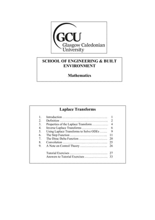
23. 22
T
t
δ ( t − T )
O
Figure 7
The Dirac delta function has the property that
.)(
,1
,0
)(
0
Ttu
Tt
Tt
dzTz
t
−=



>
<
=− δ
Another way of expressing this is that
)()( Ttu
dt
d
Tt −=−δ .
That is, the Dirac delta function is the derivative of the step function.
The Dirac delta function also has the property that
)()()(
0
TfdtTttf
M
=− δ
for any function f , providing TM > . From this result we can determine the Laplace
transform of the Dirac delta function:
.)(])([
0
Tsts
edteTtTtL −
∞
−
=−=−  δδ
The Dirac delta function is often used the model actions or events that occur over a short
period of time; reality is compressed into an instant of time for mathematical convenience. It
is sometimes referred to as the impulse function.

24. 23
Examples
(19) Solve the differential equation 5)0(,)2(34 =−=+ xtxx δ .
Transform: s
exxxs 2
34])0([ −
=+−
Substitute initial condition and solve for x :
53)4( 2
+=+ − s
exs
)4(
5
)4(
3 2
+
+
+
= −
s
e
s
x s
[A] [B]
Invert to give solution:
[A]: t
eInvert
s
4
3
)4(
3 −
+
By 2nd
Shifting Theorem,
)2(3
)4(
3 )2(42
−
+
−−−
tueInverte
s
ts
[B]: t
eInvert
s
4
5
)4(
5 −
+
tt
etuetx 4)2(4
5)2(3)( −−−
+−=
(20) In a branch of an electronic circuit, the variation of current with time is modelled by the
differential equation
dt
dV
i
dt
id
=+ 362
2
,
where )(tV is an input voltage. Suppose ])10()5([240)( −−−= tututV .
Assuming zero initial conditions, determine i as a function of t .

25. 24
Referring back to the introduction of the Dirac delta function, we can write
])10()5([240 −−−= tt
dt
dV
δδ
and so the differential equation becomes
])10()5([240362
2
−−−=+ tti
dt
id
δδ .
The Laplace transformation process results in
][
36
240 105
2
ss
ee
s
i −−
−
+
= ,
which can be inverted with the help of the 2nd
Shifting Theorem:
)10(])10(6[sin40)5(])5(6[sin40)( −−−−−= tuttutti .
Try and fill in the details for yourselves.
You may recall this warning from earlier in the notes:
The Laplace transform of a product is NOT EQUAL TO the product of the
individual Laplace transforms.
We shall now look at a kind of product rule for Laplace transforms.

26. 25
8) Convolution
The convolution of two functions )(tf and )(tg is another function of t denoted by
gf ∗ and defined by
 −=∗
t
dzzgztfgf
0
)()( [a]
or
 −=∗
t
dzztgzfgf
0
)()( . [b]
It can be shown that these two integrals are equal.
If )( sF and )( sG are the Laplace transforms of )(tf and )(tg respectively, then
)()(][ sGsFgfL =∗ .
Example
(21) Invert the Laplace transform 2
)4(
1
+ss
.
This could be done using partial fractions (try it!), but convolution could be used as an
alternative:
Set
s
sF
1
)( = and 2
)4(
1
)(
+
=
s
sG and invert individually from tables:
1)( =tf t
ettg 4
)( −
= .
Form the convolution of f and g using form [a] :
1)( =− ztf z
ezzg 4
)( −
=
.
)()(
0
4
0


−
=
−=∗
t
z
t
dzez
dzzgztfgf
Omitting the details, integration by parts gives
16
14
16
14
4
1
+−−=∗ −− tt
eetgf .

27. 26
9) A Note on Control Theory
As mentioned earlier, Laplace transforms are an important tool in control theory. Keeping
things basic, in a simple control system there may be an input and an output. Control theory
is concerned with the relationship between the input and the output within the system. Often
a control system can be modelled by a differential equation that relates input to output in what
may be referred to as the time domain. For example, a differential equation like
)(tvxk
dt
dx
=+
might relate an input )(tv to an output )(tx . For a given input, the equation is solved to
give the corresponding output. However, in control theory, options regarding the input are
often left open. Without a specific input, we can’t determine a corresponding output, but
valuable information about the systems controllability can be established by leaving the input
unspecified, and continuing to apply the solution process to the differential equation in any
case.
For the above differential equation, denote the following Laplace transforms:
)(])([ sXtxL = )(])([ sVtvL = .
Now take the Laplace transform of the differential equation; assume that the initial condition
of )(tx is zero:
)()()( sVsXksXs =+ .
Now re-arrange:
)()()( sVsXks =+
)(
1
)(
)(
kssV
sX
+
= .
What we have here is the ratio of the output of the system to its input in what is called the
Laplace domain. This ratio is called the system’s transfer function.
In general, for a system with a single input and a single output we have
)(
)(
)(
sH
sV
sX
= .
The transfer function )(sH is itself a Laplace transform and its form will depend on the
structure of the differential equation modelling the system. The transfer function plays a huge
role in control theory as much information can be derived from it. But that is another story
for another module!

28. 27
Tutorial Exercises
(1) With the aid of the table of Laplace transforms, transform the following functions :
(i) 2 5t − (ii) a t b+
(iii) 2 3 12
t t− + (iv) ( )a b t+ 2
(v) 3 t e t
(vi) t e t2 2−
(vii) e t2 1−
(viii) e tt−
cos( )2
(ix) sin( )ω θt + (x) cos( )ω θt +
(xi) sin2
t (xii) cos2
t
(xiii) e tt− 2
5sin( ) (xiv) e tt−
+2
45sin( )π
.
(2) Invert each of the following Laplace transforms :
(i)
5
3s +
(ii)
2
162
s +
(iii)
s
s
+
+
1
12
(iv)
s
s
−
−
2
42
(v)
s
s
−
−
4
42
(vi)
1
9 2
( )s +
(vii)
s
s
+
+ +
2
2 12
( )
(viii)
s
s
+
+ +
4
2 12
( )
(ix)
1
4
s
(x)
4
5
s
(xi)
s
s( )− −1 42
(xii)
5 1
1 2
s
s s
+
− +( )( )
(xiii)
s
s s
+
+ −
5
1 3( )( )
(xiv)
32
162
s s( )+
.

29. 28
(3) Using Laplace transforms, solve the following ordinary differential equations :
(i) x x+ =2 0 ; x( )0 1=
(ii) x x+ =2 1 ; x( )0 0=
(iii)  sinx x t− =3 10 ; x( )0 0=
(iv) x x− =4 0 ; x x( ) ,  ( )0 0 0 6= = −
(v) x x+ =ω 2
0 ; x A x B( ) ,  ( )0 0= =
(vi)  x x x+ + =4 4 0 ; x x( ) ,  ( )0 2 0 3= = −
(vii) 9 6 0 x x x− + = ; x x( ) ,  ( )0 3 0 1= =
(viii)  x x+ = 0 ; x x( ) ,  ( )0 0 0 4= =
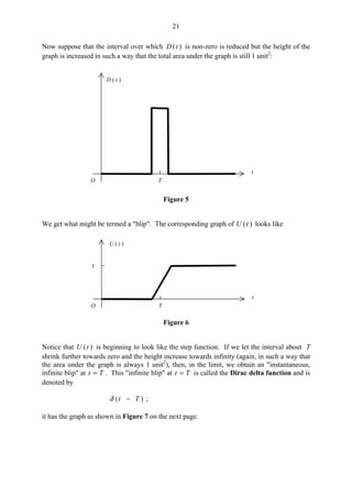
(4) Sketch the graphs and determine the Laplace transforms of each of the following :
(i) 2 5u t( )− (ii) − −4 3u t( )
(iii) 3 2 4[ ( ) ( )]u t u t− − − (iv) u t u t u t( ) ( ) ( )− − − + −1 2 2 3
(v) u t u t( ) ( )− −2 4 (vi) − − −2 3 6u t u t( ) ( )
(vii) ( ) ( )t u t− −3 3 (viii) ( ) ( )t u t− −5 52
(ix) t u t( )− 3 (x) t u t2
5( )−
(xi) [ ( ) ( )] ( )u t u t t− − − −2 4 2 2
(xii) [ ( ) ( )] ( ) [ ( ) ( )] ( )u t u t t u t u t t− − − − + − − − −1 2 1 2 3 32

30. 29
(5) Using combinations of step-functions, determine single-line expressions for each of the
following functions and (hence) their Laplace transforms :
(i)
5
2 4O
f(t)
t
(ii)
2 4O
f(t)
t
3
1
3
(iii)
2 4O
f(t)
t
3
1
3
(iv)
O
f(t)
t
5
5 10

31. 30
(v)
O
f(t)
t
5
5
(vi)
O
f(t)
t
5
5 10 15
(vii)
O
f(t)
t
5
5
(6) Invert each of the following Laplace transforms :
(i)
1
s
e s−
(ii)
1 2
s
e s−
(iii)
1
2
s
e s−
(iv)
1
2
2
s
e s−
(v)
1
2
3
s
e s
+
−
(vi)
s
s
e s
2
5
9+
−
(vii)
4
42
10
s
e s
+
−
(viii)
s
s s
e s
2
4
2 10+ +
−
(ix)
2
25
2 4
2
( )e e
s
s s− −
−
+

32. 31
(7) The ODE below models the behaviour of a time-varying current i(t) in a circuit :
di
dt
i v t+ = ( ) .
The function on the RHS, v(t) , is a source voltage. Below are various source voltages.
For each, graph v(t) and write as a single-line expression using step-functions. Then
determine and graph i(t) .
(i) v t
v t
t
( )
,
,
=
≤ ≤
≥



0 0 1
0 1
, i v( )0 0=
(ii) v t
t t
t
( )
,
,
=
≤ ≤
≥



0 1
0 1
, i( )0 0=
(8) The ODE and initial conditions
m x c x k x f t  ( )+ + = , x x( ) ( )0 0 0= =
models the mass displacement of a spring-mass-dashpot system, where m is the mass ,
c is the damping constant, k is the spring stiffness and f(t) is a forcing term. For each
of the following forcing terms graph f(t) and express it as a single-line expression .
Setting m = 1, c = 2 and k = 5, determine x in terms of t (i.e. solve the ODE).
(i) f t
t
t
( )
,
,
=
≤ ≤
≥



1 0 10
0 10
(ii) f t
t t
t
( )
,
,
=
≤ ≤
≥



0 10
0 10
(9) Evaluate the following integrals :
(i) δ ( )t dt− 1
0
2
(ii) δ ( )t dt− 3
0
2
(iii) δ ( )t dt− 1
2
4
(iv) t t dt2
0
3
2δ ( )− (v) e t dtt−
− δ ( )3
0
5
(vi) e t dtt−
− δ ( )3
0
2

33. 32
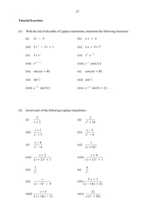
(10) Write down the Laplace transforms of
(i) 2 1δ ( )t − (ii) 4 2δ ( )t − (iii) 6 δ ( )t
(11) Invert the following Laplace transforms :
(i)
s
s
+ 1
(ii)
s
s
e s+ −1 2
(iii)
s
s
e s+
+
−2
1
4
(iv)
s s
s
e s
2
2
52
9
+
+
−
(12) Solve the following ODEs :
(i)  ( )x x t+ =4 2δ , x( )0 0=
(ii)  ( )x x t+ = −4 2 1δ , x( )0 0=
(iii)  ( )x x t+ = − −4 4δ π , x x( ) , ( )0 0 0 4= =
(iv)   ( )x x x t+ + = −4 5 1δ , x x( ) ( )0 0 0= =
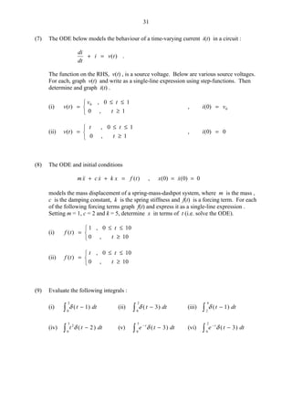
(13) The ODE and initial condition
di
dt
i v t+ = ( ) , i( )0 0=
models the behaviour of a time-varying current in a circuit. The function v(t) is a
source voltage. For each of the source voltages below, write down ( )v t ; hence
determine and graph i(t) :
(i) v t v u t( ) ( )= −0 1
(ii) v t v u t u t( ) [ ( ) ( )]= − − −0 1 2 .

34. 33
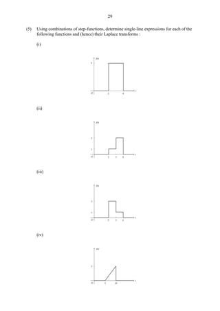
Answers
(1) (i)
2 5
2
s s
− (ii)
a
s
b
s2
+
(iii)
4 3 1
3 2
s s s
− + (iv)
a
s
ab
s
b
s
2
2
2
3
2 2
+ +
(v)
3
1 2
( )s −
(vi)
2
2 3
( )s +
(vii)
e
s
−
−
1
2
(viii)
s
s
+
+ +
1
1 42
( )
(ix)
s
s
sin cosθ ω θ
ω
+
+2 2
(x)
s
s
cos sinθ ω θ
ω
−
+2 2
(xi)
2
42
s s( )+
(xii)
s
s s
2
2
2
4
+
+( )
(xiii)
5
2 252
( )s + +
(xiv)
( ) sin cos
( )
s
s
+ +
+ +
2 5
2 25
4 4
2
π π
(2) (i) 5 3
e t−
(ii) 1
2 4sin( )t
(iii) cos sint t+ (iv) e t− 2
or cosh( ) sinh( )2 2t t−
(v) 3
2
2 1
2
2
e et t−
− (vi) t e t− 9
or
cosh( ) sinh( )2 2 2t t−
(vii) e tt− 2
cos (viii) e t tt−
+2
2( cos sin )
(ix) 1
6
3
t (x) 1
6
4
t
(xi) e t tt
[ cosh( ) sinh( ) ]2 21
2+ (xii) 2 3 2
e et t
+ −
(xiii) 2 3
e et t
− −
(xiv) 2 1 4[ cos( ) ]− t

35. 34
(3) (i) x e t
= − 2
(ii) x e t
= − −1
2
2
1( )
(iii) x e t tt
= − −3
3cos sin (iv) x t= − 3 2sinh( )
or
x e et t
= − − −3
2
2 2
( )
(v) x A t
B
t= +cos( ) sin( )ω
ω
ω (vi) x t e t
= + −
( )2 2
(vii) x et
= 3 3
(viii) x e t
= − −
4 1( )
(4) (i)
2 5
s
e s−
(ii) − −4 3
s
e s
(iii)
3 2 4
s
e es s
( )− −
− (iv)
1
2 2 3
s
e e es s s
( )− − −
− +
(v)
1 4
s
e s−
(vi) − −2 6
s
e s
(vii)
1
2
3
s
e s−
(viii)
2
3
5
s
e s−
(ix)
1 3
2
3
s s
e s
+






−
(x)
2 10 25
3 2
5
s s s
e s
+ +






−
(xi)
2 2 4 4
3
2
3 2
4
s
e
s s s
es s− −
− + +






(xii)
2 2 3 1
3 3 2
2
2
3
s
e
s s
e
s
es s s− − −
− +





 +

36. 35
(5) (i) 5 2 4[ ( ) ( )]u t u t− − −
5 2 4
s
e es s
( )− −
−
(ii) u t u t u t( ) ( ) ( )− + − − −2 2 3 3 4
1
2 32 3 4
s
e e es s s
( )− − −
+ −
(iii) 3 2 2 3 4u t u t u t( ) ( ) ( )− − − − −
1
3 22 3 4
s
e e es s s
( )− − −
− −
(iv) ( ) [ ( ) ( ) ]t u t u t− − − −5 5 10
1 1 5
2
5
2
10
s
e
s s
es s− −
− +






(v) t u t[ ( ) ]1 5− −
1 1 5
2 2
5
s s s
e s
− +






−
(vi) ( ) ( ) ( ) ( ) ( ) ( )t u t t u t t u t− − − − − + − −5 5 2 10 10 15 15
1
22
5 10 15
s
e e es s s
( )− − −
− +
(vii) ( ) [ ( ) ]5 1 5− − −t u t
5 1 1
2 2
5
s s s
e s
−





 + −

37. 36
(6) (i) u t( )− 1 (ii) u t( )− 2
(iii) ( ) ( )t u t− −1 1 (iv) ( ) ( )t u t− −2 2
(v) e u tt− −
−2 3
3( )
( ) (vi) cos[ ( )] ( )3 5 5t u t− −
(vii) 2 2 10 10sin[ ( )] ( )t u t− −
(vii) [ ]e t t u tt− −
− − − −( )
cos[ ( )] sin[ ( )] ( )4 1
33 4 3 4 4
(viii) { }2
5 5 2 2 5 4 4sin[ ( )] ( ) sin[ ( )] ( )t u t t u t− − − − −
(7) (i) i t v v e u tt
( ) [ ] ( )( )
= − − −− −
0 0
1
1 1
(ii) i t e t t u tt
( ) ( ) ( ) ( )= + − − − −−
1 1 1
(8) (i) x t f t f t u t( ) [ ( ) ( ) ( ) ]= − − −1
5 1 1 10 10
where
f t e t e tt t
1
1
21 2 2( ) cos( ) sin( )= − −− −
(ii) x t g t g t u t g t u t( ) ( ) ( ) ( ) ( ) ( )= − − − − − −1 1 210 10 2 10 10
where
[ ]g t t e t e tt t
1
1
25
3
25 2 2 2 2( ) cos( ) sin( )= − + −− −
g t e t e tt t
2
1
21 2 2( ) cos( ) sin( )= − −− −

38. 37
(9) (i) 1 (ii) 0 (iii) 0
(iv) 4 (v) e − 3
(vi) 0
(10) (i) 2 e s−
(ii) 4 2
e s−
(iii) 6
(11) (i) δ ( )t + 1
(ii) δ ( ) ( )t u t− + −2 2
(iii) δ ( ) ( )( )
t e u tt
− + −− −
4 44
(iv) δ ( ) { cos[ ( )] sin[ ( )]} ( )t t t u t− + − − − −5 2 3 5 3 3 5 5
(12) (i) x t e t
( ) = −
2 4
(ii) x t e u tt
( ) ( )( )
= −− −
2 14 1
(iii) x t t u t( ) sin( ) [ ( )]= − −2 2 1 π
(iv) x t e t u tt
( ) sin( ) ( )( )
= − −− −2 1
1 1
(13) (i) i t v e u tt
( ) ( )( )
= −− −
0
1
1
(ii) i t v e u t e u tt t
( ) [ ( ) ( ) ]( ) ( )
= − − −− − − −
0
1 2
1 2

39. 38

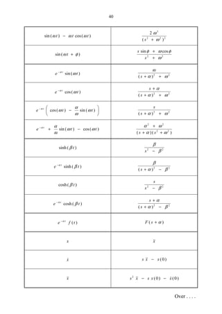
40. 39
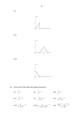
TABLE OF LAPLACE TRANSFORMS
])([ tfL is defined by dtetf ts

∞
−
0
)(
)(tf ])([)( tfLsF =
1
s
1
t 2
1
s
2
t 3
2
s
n
t 1
!
+n
s
n
t
e α−
)(
1
α+s
t
et α−
2
)(
1
α+s
t
e α−
−1
)( α
α
+ss
)(sin tω 22
ω
ω
+s
)(cos tω 22
ω+s
s
)(cos1 tω−
)( 22
2
ω
ω
+ss
)(sin tt ωω 222
2
)(
2
ω
ω
+s
s
Over . . . .

41. 40
)(cos)(sin ttt ωωω − 222
3
)(
2
ω
ω
+s
)(sin φω +t 22
cossin
ω
φωφ
+
+
s
s
)(sin te t
ωα−
22
)( ωα
ω
++s
)(cos te t
ωα−
22
)( ωα
α
++
+
s
s






−−
)(sin)(cos tte t
ω
ω
α
ωα
22
)( ωα ++s
s
)(cos)(sin tte t
ωω
ω
αα
−+−
)()( 22
22
ωα
ωα
++
+
ss
)(sinh tβ 22
β
β
−s
)(sinh te t
βα−
22
)( βα
β
−+s
)(cosh tβ 22
β−s
s
)(cosh te t
βα−
22
)( βα
α
−+
+
s
s
)(tfe tα−
)( α+sF
x x
x )0(xxs −
x )0()0(2
xxsxs −−
Over . . . .

42. 41
Unit Step Function



>
<
=−
Tt
Tt
Ttu
,1
,0
)( Ts
e
s
−1
)()( TtuTtf −− Ts
esF −
)(
Dirac Delta Function
)(tδ 1
)( Tt −δ Ts
e −
Convolution Integral


−
−
t
t
dzzgztf
dzztgzf
0
0
)()(
OR
)()(
)()( sGsF